8. Logistic Regression
Multiple and Logistic Regression 1
- 4 conditions for logistic regression:
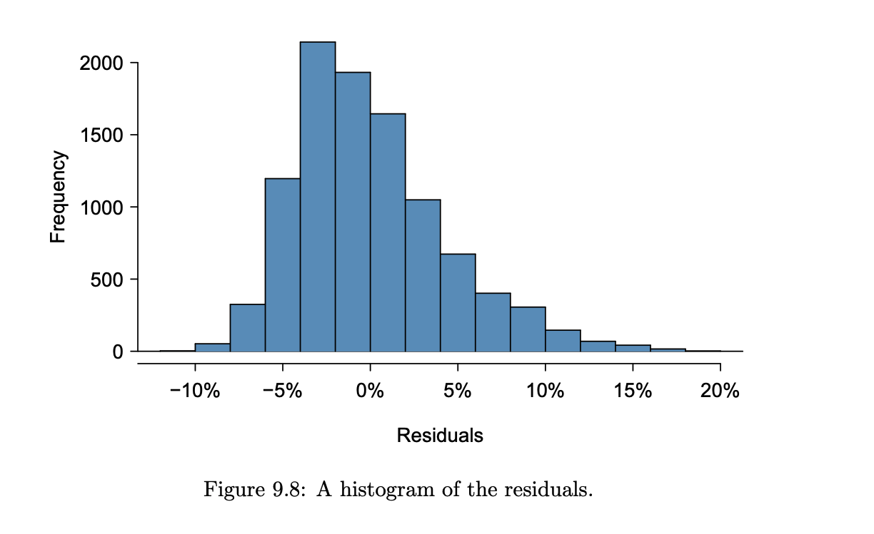
- (1)- Residuals are nearly normal.
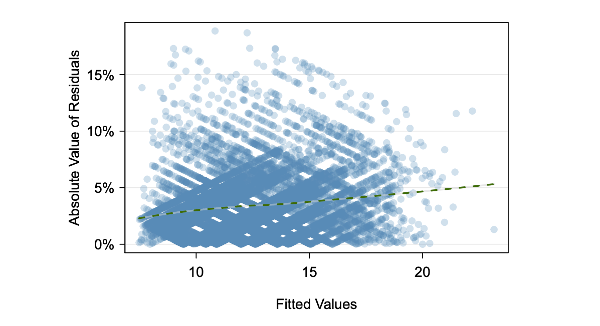
- (2)- Variability of residuals is nearly constant.
- (3)- Residuals are independent.
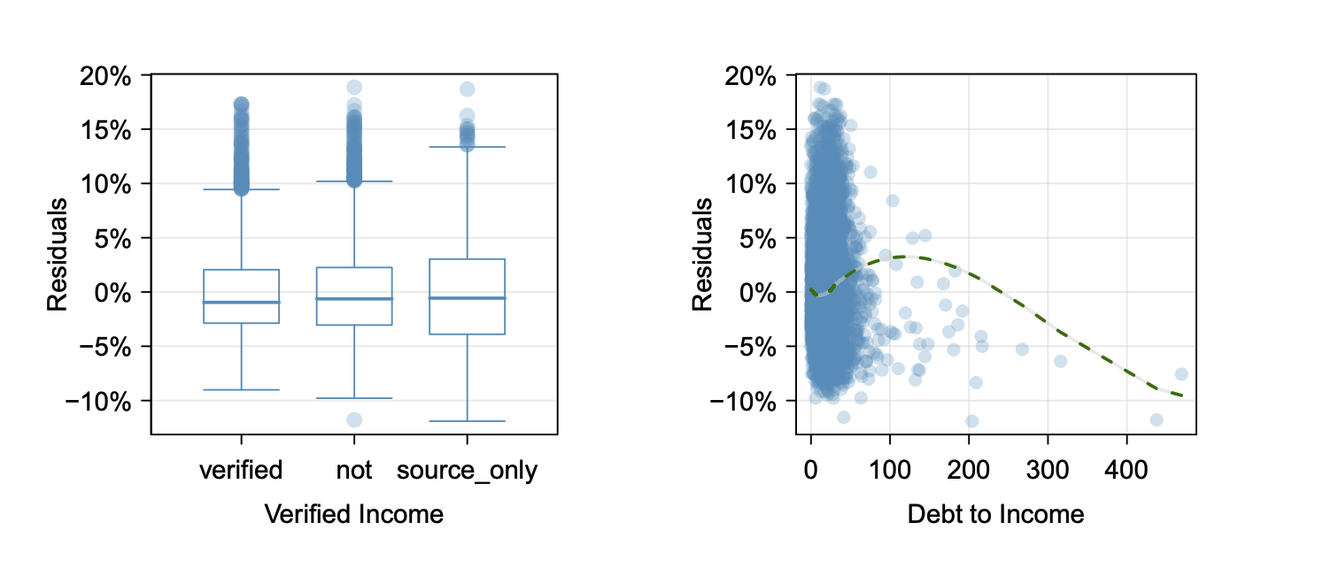
- (4)- Each variable is linearly related to the outcome.
- Diagnostic plots are used to check these conditions.
| (1)- Check for outliers (normality) | Histogram of residuals |  |
| (2)- Check variance of residuals is constant | Absolute values of the residuals against fitted (predicted) values |  |
| (3)- Check No patterns in residuals. | Residuals in order of their data collection or Time series | |
| (4)- Check linearity in relation to outcome | Residuals against each predictor variable |  |
Logistic Regression in JASP 2
- The null hypothesis tested is that there is no relationship between the outcome and the predictor variable(s).
- sigmoidal logistic regression curve is fitted with a minimum of 0 and a maximum of 1.
- The confusion matrix is a table showing actual vs predicted outcomes and can be used to determine the accuracy of the model. From this sensitivity and specificity can be derived.
- Sensitivity is the percentage of cases that had the observed outcome was correctly predicted by the model (i.e., true positives).
- Specificity is the percentage of observations that were also correctly predicted as not having the observed outcome (i.e., true negatives).
Checking model conditions using graphs 3
- Assumptions of logistic regression:
- Residuals of the model are nearly normally distributed.
- variability of the residuals is nearly constant across all values of the predictor variable.
- Residuals are independent of each other.
- Each variable is linearly related to the outcome.
Basic ideas of logistic regression 4
- It is used when the outcome variable is binary.
- It is a type of generalized linear model (GLM) where regular multiple regression does not work.
- The result takes two possible values, 0 or 1; with \(p_i\) being the probability of the outcome being 1; Hence:
- The probability of the outcome being 1 is \(p_i\).
- The probability of the outcome being 0 is \(1 - p_i\).
- Two key conditions for fitting a logistic regression model:
- The model relating the parameter \(p_i\) to the predictors \(x_{1,i}, x_{2,i}, \ldots, x_{k,i}\) must closely resemble the true relationship between the predictors and the parameter.
- The outcome for each case must be independent of the outcome for all other cases.
- Evaluate the independence assumption by examining the residuals for patterns:
- \(e_i = Y_i - \hat{p}_i\)
How to perform a logistic regression analysis in JASP 5
- From the JASP menu, select
Regressionand thenLogistic Regression. - Drag the dependent (outcome) variable to the
Dependent Variablebox. - Drag the independent (predictor) variable to the
CovariatesandFactorsboxes.- For categorical predictors, drag them to the
Factorsbox. - For continuous predictors, drag them to the
Covariatesbox.
- For categorical predictors, drag them to the
- Under
Statistics>Regression Coefficients, selectOdds Ratiosto get the odds ratios for the predictors. - Under
Plots, selectDisplay conditional estimates plotto get the predicted probabilities for the predictors. - Under
Statistics:- From
Performance Diagnostics, selectConfusion Matrixto get the confusion matrix. - From
Performance metrics:- Select
Sensitivitywhich describes the proportion of true positives. - Select
Specificitywhich describes the proportion of true negatives.
- Select
- From
References
-
Diez, D. M., Barr, C. D., & Çetinkaya-Rundel, M. (2019). Openintro statistics - Fourth edition. Open Textbook Library. https://www.biostat.jhsph.edu/~iruczins/teaching/books/2019.openintro.statistics.pdf Read Chapter 9 - Multiple and logistic regression Section 9.3 - Checking model conditions using graphs from page 358 to 364 Section 9.5 – Introduction to logistic regression from page 371 to 383 Solve the following practice exercises as homework from the attached: Practice Exercises Unit 8.pdf ↩
-
Goss-Sampson, M. A. (2022). Statistical analysis in JASP: A guide for students (5th ed., JASP v0.16.1 2022). https://jasp-stats.org/wp-content/uploads/2022/04/Statistical-Analysis-in-JASP-A-Students-Guide-v16.pdf Read Logistic Regression from page 86 to 90. ↩
-
OpenIntroOrg. (2013a, November 24). Checking multiple regression diagnostics using graphs [Video]. YouTube. https://youtu.be/3KSUeYMKt5A ↩
-
OpenIntroOrg. (2013b, November 30). Basic ideas of logistic regression [Video]. YouTube. https://youtu.be/uYC2eLVSpI8 ↩
-
JASP Statistics. (2018, February 11). How to perform a logistic regression analysis in JASP [Video]. YouTube. https://youtu.be/bUgpJeeReBY ↩