WA4. Classification Exercise
K-NEAREST NEIGHBORS EXERCISE – ASSIGNMENT UNIT 4
Imaging objects in classes A and B having two numeric attributes/properties that we map to X and Y Cartesian coordinates so that we can plot class instances (cases) as points on a 2-D chart. In other words, our cases are represented as points with X and Y coordinates (p(X,Y)).
Our simple classes A and B will have 3 object instances (cases) each.
Class A will include points with coordinates (0,0), (1,1), and (2,2). Class B will include points with coordinates (6,6), (5.5, 7), and (6.5, 5).
In R, we can write down the above arrangement as follows:
- Class A training object instances (cases):
- A1=c(0,0)
- A2=c(1,1)
- A3=c(2,2)
-
Class B training objects instances (cases)
- B1=c(6,6)
- B2=c(5.5,7)
- B3=c(6.5,5)
-
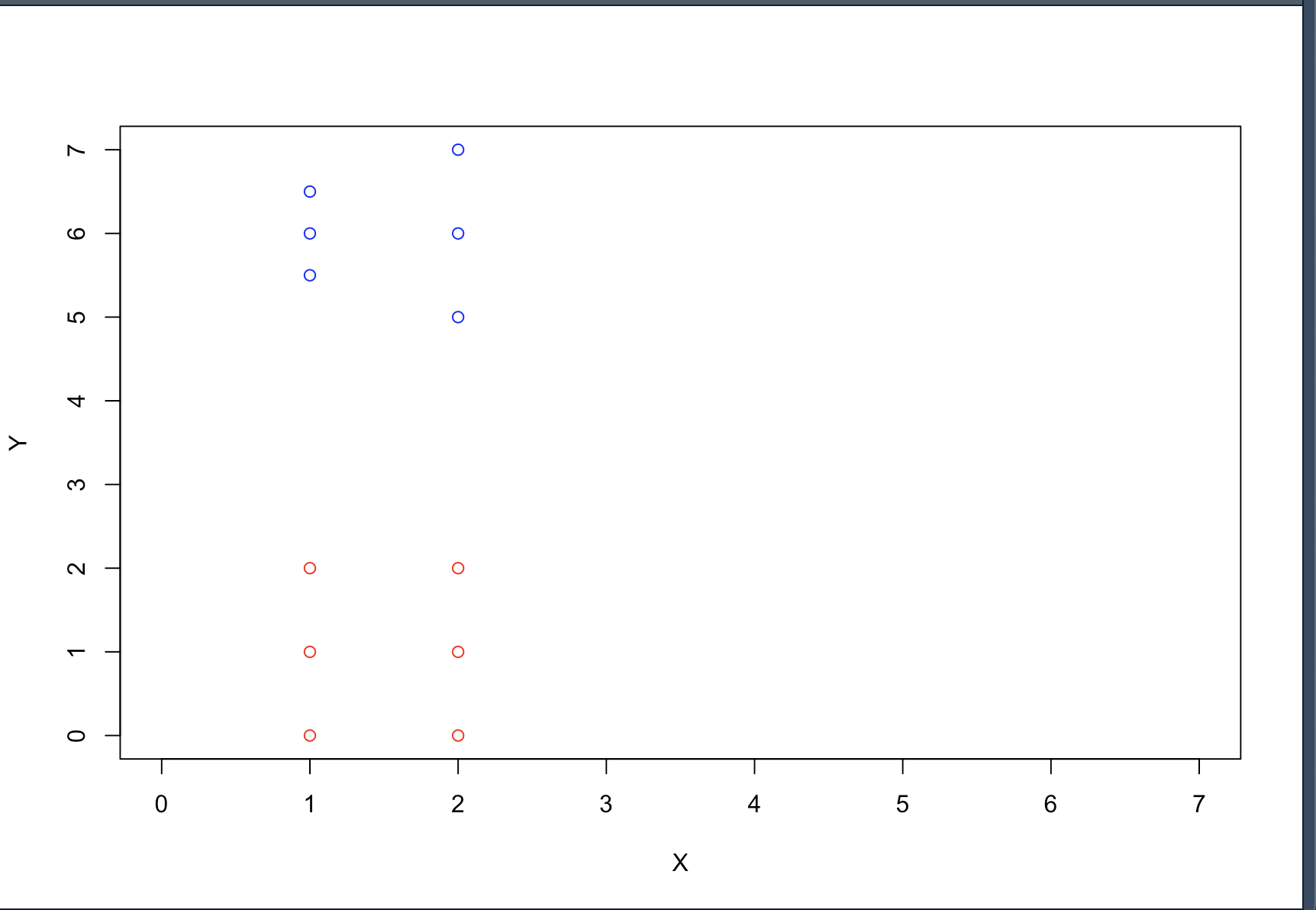
How are the classification training objects for class A and class B arranged on a chart?.
- Print the chart.
# Class A training object instances (cases):
A1=c(0,0)
A2=c(1,1)
A3=c(2,2)

# Class B training objects instances (cases)
B1=c(6,6)
B2=c(5.5,7)
B3=c(6.5,5)

# How are the classification training objects for class A
# and class B arranged on a chart?
plot(A1, col="red", xlim=c(0,7), ylim=c(0,7), xlab="X", ylab="Y")
points(A2, col="red")
points(A3, col="red")
points(B1, col="blue")
points(B2, col="blue")
points(B3, col="blue")

The knn() function is housed in the class package and is invoked as follows: knn(train, test, cl, k) where
- train is a matrix or a data frame of training (classification) cases.
- test is a matrix or a data frame of test case(s) (one or more rows).
- cl is a vector of classification labels (with the number of elements matching the number of classes in the training data set).
- k is an integer value of closest cases (the k in the k-Nearest Neighbor Algorithm); normally, it is a small odd integer number.
Now, when we try out classification of a test object (with properties expressed as X and Y coordinates), the kNN algorithm will use the Euclidean distance metric calculated for every row (case) in the training matrix to find the closest one for k=1 and the majority of closest ones for k > 1 (where k should be an odd number).
- Construct the cl parameter (the vector of classification labels).
# Construct the cl parameter (the vector of classification labels)
cl <- c("A", "A", "A", "B", "B", "B")
To run the knn() function, we need to supply the test case(s), which corresponds to a point sitting approximately in the middle of the distance between A and B. suppose test=c(4,4).
At this point, we have everything in place to run knn(). Let’s do it for k = 1 (classification by its proximity to a single neighbor).
For more informative reports of test object classification results, we are going to use the summary() function that can polymorphically act on its input parameter depending on its type. In our case, the input parameter to the summary() function is the output of the knn() function.
- Calculate summary() function of knn() and show the results
# Construct the train and test parameters
train <- rbind(A1, A2, A3, B1, B2, B3)
test <- c(4,4)

# Calculate summary() function of knn() and show the results
summary(knn(train, test, cl, k=1))
The output of the summary() function is as follows:

The results above indicates that the tested object (4,4) is classified as B (1 item identified as B, 0 items identified as A).
- Which class does the test case belong to?
Class B.
Now define test=c(3.5, 3.5) Visually, this test case point looks to be closer to the cluster of the A class cases (points)
- Calculate summary() function of knn() and show the results
The summary() function output is as follows:

The results above indicates that the tested object (3.5,3.5) is classified as A.
- Which class does the test case now belong to?
Class A.
Let’s increase the number of closest neighbors that are involved in voting during the classification step.
- Calculate the summary using K=3 and tell which class does the test case belong to?
test35 <- c(3.5,3.5)
test44 <- c(4,4)
k=3


# summary of (4,4)
summary(knn(train, test44, cl, k))

#  summary of (3.5,3.5)
summary(knn(train, test35, cl, k))
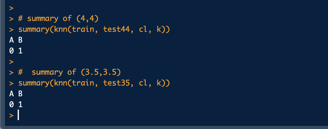
The summary() function output is as follows:

We notice that both test cases are classified as B.
So the point (3.5,3.5) has flipped sides and is now classified as B.
Now, let’s build a matrix of test cases containing four points:
- T1=(4,4)
- T2=(3,3)
- T3=(5,6)
-
T4=(7,7)
-
Create test as a two-column matrix containing the X and Y coordinates of our test points.
# Construct the test matrix
testMatrix <- matrix(c(4,4,3,3,5,6,7,7), nrow=4, byrow=TRUE)
- Now run again the previous knn summary command and show the results.
# run the knn summary for each element in the test matrix
summary(knn(train, test=testMatrix, cl, k))
And the output is as follows:

- How many of the points in our test batch are classified as belonging to each class?
We notice that 3 points are classified as B and 1 point is classified as A.
Here is the complete code:
library(class)

# Class A training object instances (cases):
A1=c(0,0)
A2=c(1,1)
A3=c(2,2)

# Class B training objects instances (cases)
B1=c(6,6)
B2=c(5.5,7)
B3=c(6.5,5)

# How are the classification training objects for class
# A and class B arranged on a chart?
plot(A1, col="red", xlim=c(0,7), ylim=c(0,7), xlab="X", ylab="Y")
points(A2, col="red")
points(A3, col="red")
points(B1, col="blue")
points(B2, col="blue")
points(B3, col="blue")

cl <- c("A", "A", "A", "B", "B", "B")

# Construct the train parameter (the matrix of training cases)
train <- rbind(A1, A2, A3, B1, B2, B3)
test35 <- c(3.5,3.5)
test44 <- c(4,4)
k=3


# summary of (4,4)
summary(knn(train, test44, cl, k))

#  summary of (3.5,3.5)
summary(knn(train, test35, cl, k))


# Construct the test matrix
testMatrix <- matrix(c(4,4,3,3,5,6,7,7), nrow=4, byrow=TRUE)


# run the knn summary for each element in the test matrix
summary(knn(train, test=testMatrix, cl, k))