7. Interpolation and Spline Modeling
Introduction 1
- Linear interpolation: connecting two vertices with a straight line.
- Anti-aliasing can be used to adjust the position and intensity of some of the pixels within the model to smooth the line.
- Interpolating a spline is a bit more complex.
- In the linear model, we are using some variation of the equation of a line to compute the position of pixels that exist between the two vertices.
- In a spline, we select a series of control points (2 or more), and a curve is fitted within these control points based upon the particular algorithm used.
Bezier Curves and Splines 2
- PolyLines: a sequence of vertices connected by straight line segments.
- Smooth curves: a sequence of vertices connected by curves.
- Splines:
- A sequence of vertices connected by curves based on a set of control points.
- A special type of smooth curve in 2D or 3D space.
- Use cases:
- 2D illustrations.
- Fonts.
- Animation: trajectory of objects.
- Definitions of Curves:
- A curve is a continuos 1D set of points in 2D or 3D space.
- A curve is a mapping from an interval S onto a plane.
- Two approaches: Interpolation and Approximation:
- Interpolation goes through all control points, while approximation may skip some.
- Interpolation is more complex and less stable, while approximation is more convenient.
- Why interpolation is useful:
- Good for UI: smooth curves.
- Good for storage: only store control points.
- Tessellation:
- The process of breaking down a curve into a series of straight lines.
- Cubic Bézier Curve:
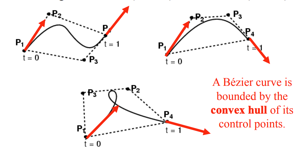
- It is a curve defined by four control points (P1, P2, P3, P4).
- The curve starts at P1 and ends at P4.
- The curve may not pass through P2 and P3.
- The equation is cubic polynomial.
- Curve is tangent at P1 to (P1-P2) and at P4 to (P4-P3).

- P(t) is a weighted combination of the 4 control points with weights:
- \(B1(t) = (1-t)^3\)
- \(B2(t) = 3t(1-t)^2\)
- \(B3(t) = 3t^2(1-t)\)
- \(B4(t) = t^3\)
- First P is the most influential, as P1 > P2 > P3 > P4 in their influence.
- The basis polynomials/vectors are Bernstein polynomials (4X1 vectors).
- \(P(t) = P1B1(t) + P2B2(t) + P3B3(t) + P4B4(t) = \sum_{i=1}^{4} P_iB_i(t)\)
- Bezier Curves of degree n:
- \(P(t) = \sum_{i=0}^{n} P_iB_i(t)\)
- We can find the equation of a Bezier curve of any degree, if we know n, and i according to:

- \(B_i^n(t) = \frac{n!}{i! (n-i)!}t^i(1-t)^{n-1}\)
Curves Properties and Conversion, Surface Representation 2
- Linear Transformations & Cubics:
- We transform the control points of a cubic Bezier curve using a linear transformation matrix.
- Because everything is linear, it is the same as transforming only the control points.
- Continuity:
- Parametric continuity condition represents that how smoothly a curve transit from one curve segment to another segment.
- Read https://www.geeksforgeeks.org/parametric-geometric-continuity-of-curves-in-computer-graphics/
- Also read https://people.eecs.berkeley.edu/~jfc/cs184f98/lec19/lec19.html
- Orders of Continuity:
- C0: Continuous: two segments meet at the same point.
- G1: Geometric continuity: two segments tangents with the same direction.
- C1: Parametric continuity: two segments tangent at the same point and their first derivatives are the same (implies G1).
- C2: Curvature continuity: two segments tangents and their first and second derivatives are the same.
- Parametric surface P(u,v):
- It is a bicubic polynomial of two variables u & v.
- Defined by 4x4=16 control points P1,1, P1,2.... P4,4.
- Basis are product of two Bernstein polynomials: B1(u)B1(v); B1(u)B2(v);… B4(u)B4(v).
- Interpolates 4 corners, approximates others.
- It turns out corner cutting (Chaikin’s Algorithm) produces a quadratic BSpline curve.
Interactive Introduction to Splines 3
Bezier Spline Curves
- Linear Bezier spline:
- It is a linear interpolation between two points. P0 and P1.
- \(P(t) = (1-t)P0 + tP1\) for \(0 \leq t \leq 1\).
- It is a straight line starts at P0 and ends at P1.
- Quadratic Bezier spline:
- It is a quadratic interpolation between three points. P0, P1, and P2.
- Cubic Bezier spline:
- It is a cubic interpolation between four points. P0, P1, P2, and P3.
- It is a curve that starts at P0 and ends at P3.
Interpolation and Spline Modeling 4
- Interpolation:
- It is a method of constructing new data points within the range of a discrete set of known data points.
- Example: given a set of a few points that belongs to a curve, we can interpolate the curve to find the points in between.
- Algorithms of Interpolation:
- Bernstein, Bezier. and Catmull-Rom.
- All of them are equations that can be used to interpolate a curve based on some parameters and a set of points.
- Spline:
- A spline is a curve that is defined by a set of control points and a set of basis functions that are used to interpolate the curve.
- It is obtained by DeCasteljau algorithm.
References
-
Learning Guide Unit 7: Introduction | Home. (2024). Uopeople.edu. https://my.uopeople.edu/mod/book/view.php?id=444306&chapterid=540625 ↩
-
Massachusetts Institute of Technology (2020). Coordinates and Transformations. MITOpenCourseware. https://ocw.mit.edu/courses/electrical-engineering-and-computer-science/6-837-computer-graphics-fall-2012/lecture-notes/. (Original work published 2001). Read Lecture #1: Bezier Curves and Splines. Read Lecture #2: Curves Properties and Conversion, Surface Representation. ↩↩
-
An Interactive Introduction to Splines. (2021). Ibiblio.org. https://www.ibiblio.org/e-notes/Splines/Intro.htm ↩
-
Unit 7 Lecture 1: Interpolation and Spline Modeling | Home. (2024). Uopeople.edu. https://my.uopeople.edu/mod/kalvidres/view.php?id=444312 ↩