WA5. Decision Trees Lab
Statement
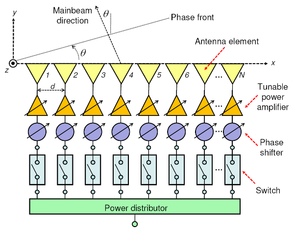
This radar data was collected by a system in Goose Bay, Labrador. This system consists of a phased array of 16 high-frequency antennas with a total transmitted power on the order of 6.4 kilowatts. See the paper for more details. The targets were free electrons in the ionosphere.

- “Good” radar returns are those showing evidence of some type of structure in the ionosphere.
- “Bad” returns are those that do not; their signals pass through the ionosphere.
Received signals were processed using an autocorrelation function whose arguments are the time of a pulse and the pulse number. There were 17 pulse numbers for the Goose Bay system. Instances in this database are described by 2 attributes per pulse number, corresponding to the complex values returned by the function resulting from the complex electromagnetic signal.
Part 1: Print decision tree:
- a. We begin by setting the working directory, loading the required packages (rpart and mlbench) and then loading the Ionosphere dataset.
- b. Use the rpart() method to create a regression tree for the data.
- c. Use the plot() and text() methods to plot the decision tree.
Part 2: Estimate accuracy:
- a. Split the data a test and train subsets using the sample() method.
- b. Use the rpart method to create a decision tree using the training data.
- c. Use the predict method to find the predicted class labels for the testing data.
- d. Use the table method to create a table of the predictions versus true labels and then compute the accuracy. The accuracy is the number of correctly assigned good cases (true positives) plus the number of correctly assigned bad cases (true negatives) divided by the total number of testing cases.
Solution
Part 1: Print decision tree
The following R code summarizes the process, please follow comments for details.
# loading necessary libraries
library(rpart)
library(mlbench)

# loading the dataset
Ionosphere <- read.csv("wa5.data.csv", header = FALSE)
data(Ionosphere)

# build the decision tree
tree <- rpart(Class ~ ., data = Ionosphere, method = "class")

# plot the decision tree
plot(tree)
text(tree, use.n = TRUE, all = TRUE, cex = 0.8)
And the resulting decision tree is shown below:
However, the tree above is not very pretty, So I used other libraries called rpart.plot, rattle and RColorBrewer to plot a nicer tree, shown below using the following R code:
# Plot the tree
library(rattle)
library(rpart.plot)
library(RColorBrewer)


# plot the tree
fancyRpartPlot(
    tree,
    palettes = c("Reds", "Greens", "Oranges"),
    caption = "Decision Tree For Ionosphere Data"
)
Part 2: Estimate accuracy
a. Split the data a test and train subsets using the sample() method
The following R code splits the data into training and testing sets:
# Split the data into training and testing sets
train_indices <- sample(
    seq_len(nrow(Ionosphere)),
    0.7 * nrow(Ionosphere)
)
train_set <- Ionosphere[train_indices, ]
test_set <- Ionosphere[-train_indices, ]
The data is split into 70% training and 30% testing sets, where according to (R Documentation, n.d.):
sample()takes a sample of the specified size from the elements of a set using either with or without replacement.nrow()returns the number of rows in the data.seq_len(l)returns a sequence of integers from 1 tol, but it is safe if l is smaller than 1.
b. Use the rpart method to create a decision tree using the training data
# build the decision tree of the training data
tree_train <- rpart(
    Class ~ .,
    data = train_set,
    method = "class"
)
c. Use the predict method to find the predicted class labels for the testing data.
# predict the class labels for the testing data
pred <- predict(
    tree_train,
    newdata = test_set,
    type = "class"
)
d. Use the table method to create a table of the predictions versus true labels and then compute the accuracy
# create a table of the predictions versus true labels
result <- table(pred, test_set$Class)

# compute the accuracy
accuracy <- sum(diag(result)) / sum(result)
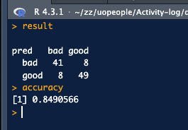
We get the following result:

And numerically, the accuracy is:
| pred | Bad | Good |
|---|---|---|
| Bad | 41 | 8 |
| Good | 8 | 49 |
Which means that:
- The model correctly predicted 49 good cases (true positives).
- The model correctly predicted 41 bad cases (true negatives).
- The model incorrectly predicted 8 bad cases (false positives).
- The model incorrectly predicted 8 good cases (false negatives).
The accuracy is then:
> accuracy
[1] 0.8490566
let’s compute the accuracy manually:
accuracy = (true positives + true negatives) / (total cases)
         =  (49 + 41) / (49 + 41 + 8 + 8)
         = 0.8490566
Thus accuracy is 84.9%.
R Code
Here is all the R, code in a single snippet, please make sure that you install all missing libraries before running the code.
# read data.csv file
Ionosphere <- read.csv("wa5.data.csv", header = FALSE)


library(rpart)
library(mlbench)
data(Ionosphere)


tree <- rpart(Class ~ ., data = Ionosphere, method = "class")

# Plot the tree
# plot(tree)
# text(tree, use.n = TRUE, all = TRUE, cex = 0.8)

library(rattle)
library(rpart.plot)
library(RColorBrewer)


# plot the tree
fancyRpartPlot(
    tree,
    palettes = c("Reds", "Greens", "Oranges"),
    caption = "Decision Tree For Ionosphere Data"
)


# Split the data into training and testing sets
train_indices <- sample(
    seq_len(nrow(Ionosphere)),
    0.7 * nrow(Ionosphere)
)

train_set <- Ionosphere[train_indices, ]
test_set <- Ionosphere[-train_indices, ]


# build the decision tree of the training data
tree_train <- rpart(
    Class ~ .,
    data = train_set,
    method = "class"
)

# predict the class labels for the testing data
pred <- predict(
    tree_train,
    newdata = test_set,
    type = "class"
)


# create a table of the predictions versus true labels
result <- table(pred, test_set$Class)

# compute the accuracy
accuracy <- sum(diag(result)) / sum(result)
References
- R Documentation (n.d.). R Documentation. https://www.rdocumentation.org/
- James, G., Witten, D., Hastie, T., & Tibshirani, R. (2013). An introduction to statistical learning with applications in R. New York, NY: Springer. Read Chapter 8: Tree-Based Methods, p. 303-335.
- Gorman B. (2014). Decision Trees in R using rpart. GormAnalysis. https://www.gormanalysis.com/blog/decision-trees-in-r-using-rpart/
- Awati K. (2016). A gentle introduction to decision trees using R. https://eight2late.wordpress.com/2016/02/16/a-gentle-introduction-to-decision-trees-using-r/