JA4. Exercises
Problem 1

A survey of high school seniors was conducted by the National Center of Education Statistics. They were collecting test data on reading, writing, and several other subjects. A random sample of 250 students was examined from the survey. Side-by-side box plots of reading and writing scores as well as a histogram of the differences in scores are shown below.
(a) Create hypotheses appropriate for the following research question: is there an evident difference in the average scores of students in the reading and writing exam?.
The two data sets are paired due to the same students may take both exams which makes observations somehow dependent on each other. Therefore, we will use a paired T-test (Cetinkaya-Rundel, 2018).
- H0: null hypothesis: There is no difference in the average scores of students in the reading and writing exam. \(\mu_{diff} = 0\).
- Ha: alternative hypothesis: There is a difference in the average scores of students in the reading and writing exam, that is, positive or negative difference. \(\mu_{diff} ≠ 0\).
Note: that diff denotes the difference between the reading and writing scores, which is denoted as read-write in the question.
(b) Check the conditions required to complete this test.
There are two main conditions to check before performing a paired T-test, collected from the OpenIntro Statistics textbook (Diez, Barr, & Çetinkaya-Rundel, 2019, p.251) and Cetinkaya-Rundel (2018):
- Independence Test:
- Random assignment: The students were randomly selected, so this condition is satisfied.
- 10% condition: The sample size is less than 10% of the population (250 students out of all high school seniors), so this condition is satisfied.
- Sample Size/Right-Skewed Test (Normality):
- The sample size is large enough (n = 250 >= 30) to use the T-distribution for the test.
- From the provided histogram, there are no extreme outliers, so the data is not too skewed.
- The histogram also shows an approximately normal distribution, so the normality condition is satisfied.
Since the conditions are satisfied, we can proceed with the hypothesis test using a paired T-test.
c) The average observed difference in scores is and \(\overline{x}_{read-write=-0.545,}\) , and the standard deviation of the differences is 8.887 points. Do these data provide convincing evidence of a difference between the average scores on the two exams?.
◦ Calculate the T-test.
◦ Calculate the degrees of freedom.
◦ Given the p-value of 0.39, provide the conclusion.
The p-value = 0.39 is greater than the significance level of 0.05. Therefore, we fail to reject the null hypothesis.
We accept the null hypothesis, and we conclude that there is not enough evidence to suggest that there is a difference between the average scores on the two exams.
(d) What type of error might we have made? Explain what the error means in the context of the application.
We failed to reject the null hypothesis, and accepted it; it is possible that the null hypothesis is false but we have mistakenly accepted is true. This is a Type II error.
In the context of the application, it is possible that there is in fact a difference between the average scores on the two exams, but we failed to detect it as we concluded that there is no difference.
(e) Based on the results of this hypothesis test, would you expect a confidence interval for the average difference between the reading and writing scores to include 0? Explain your reasoning.
Let’s calculate the confidence interval based on the information provided:
Note: The t-score of 1.97 is obtained with a 95% confidence level and 249 degrees of freedom using the tool at this website: https://homepage.divms.uiowa.edu/~mbognar/applets/t.html
The confidence interval is (-1.652, 0.562). We have a 95% confidence that the true difference in the average scores between the reading and writing exams is between -1.652 and 0.562. 0 is clearly within the confidence interval.
Another way to look at this as we failed to reject the null hypothesis that says the average difference in scores is 0. Therefore, we would expect that value (0) to be within the confidence interval.
Problem 2
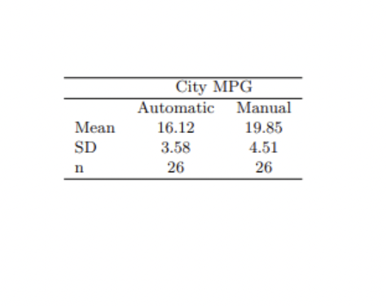
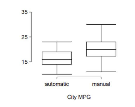
Each year the US Environmental Protection Agency (EPA) releases fuel economy data on cars manufactured in that year. Below are summary statistics on fuel efficiency (in miles/gallon) from random samples of cars with manual and automatic transmissions.


Do these data provide strong evidence of a difference between the average fuel efficiency of cars with manual and automatic transmissions in terms of their average city mileage? Assume that conditions for inference are satisfied.
(1) State the hypothesis.
The two data sets are independent, as the type of transmission in a car does not affect the other. Therefore, we will use a two-sample T-test (Cetinkaya-Rundel, 2018).
We will be denoting the average fuel efficiency of manual cars as \(\mu_{m}\) and automatic cars as \(\mu_{a}\).
- H0: null hypothesis: There is no difference in the average fuel efficiency between manual and automatic cars. \(\mu_{m} = \mu_{a}\) or \(\mu_{m} - \mu_{a} = 0\).
- Ha: alternative hypothesis: There is a difference in the average fuel efficiency between manual and automatic cars. \(\mu_{m} ≠ \mu_{a}\) or \(\mu_{m} - \mu_{a} ≠ 0\).
(2) Calculate the T-statistics.
let’s compute the standard error first:
Now, we can calculate the T-statistics:
(3) Calculate the degrees of freedom.
The degrees of freedom can be calculated using the formula (Cetinkaya-Rundel, 2018):
(4) Given the p-value of 0.0029, provide a conclusion to the hypothesis test.
The p-value = 0.0029 is less than the significance level of 0.05. Therefore, we reject the null hypothesis. And we accept the alternative hypothesis, that is, there enough evidence to suggest that there is a difference in the average fuel efficiency between manual and automatic cars.
References
- Cetinkaya-Rundel, M. (2018). 5 2 Inference for paired data [YouTube Video]. In YouTube. https://www.youtube.com/watch?v=K0QZ9_4w0HU
- Diez, D. M., Barr, C. D., & Çetinkaya-Rundel, M. (2019). Openintro statistics - Fourth edition. Open Textbook Library. https://www.biostat.jhsph.edu/~iruczins/teaching/books/2019.openintro.statistics.pdf Chapter 7 - Inference for numerical data.