6. Introduction to Linear Regression

Introduction to Linear Regression ¹

Statistical Analysis in JASP: A guide for students ²

Line fitting, residuals, and correlation ³

• Linear regression assumes that a relationship between two variables can be described by a straight line.
• The perfect linear relationship between two variables is rare in practice, but it means that you can know the exact value of one variable if you know the exact value of the other variable.
• \(y = \beta_0 + \beta_1x\) where \(y\) is the response variable, \(x\) is the explanatory variable, \(\beta_0\) is the y-intercept, and \(\beta_1\) is the slope.
• b0, b1 are the estimates of the population parameters \(\beta_0\) and \(\beta_1\).
• Residuals are the differences between the observed values of the response variable and the values predicted by the regression line.
• Data = Fit + Residuals.
• Residual is the difference between the observed value and the predicted value (the value on the line).
• If the point is above the line, the residual is positive, and if the point is below the line, the residual is negative.
• The line is chosen in way that minimizes the sum of the residuals.
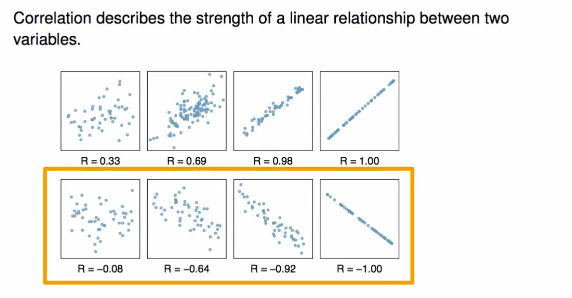
• Correlation measures the strength and direction of the linear relationship between two variables.
• Correlation is always between -1 and 1.
• Upward sloping line has a positive correlation, and downward sloping line has a negative correlation.
• As observations move closer to the line, the residuals decrease, and correlation increases.
• 

Fitting a line with least squares regression ⁴

• The least squares regression line is the line that minimizes the sum of the squared residuals.
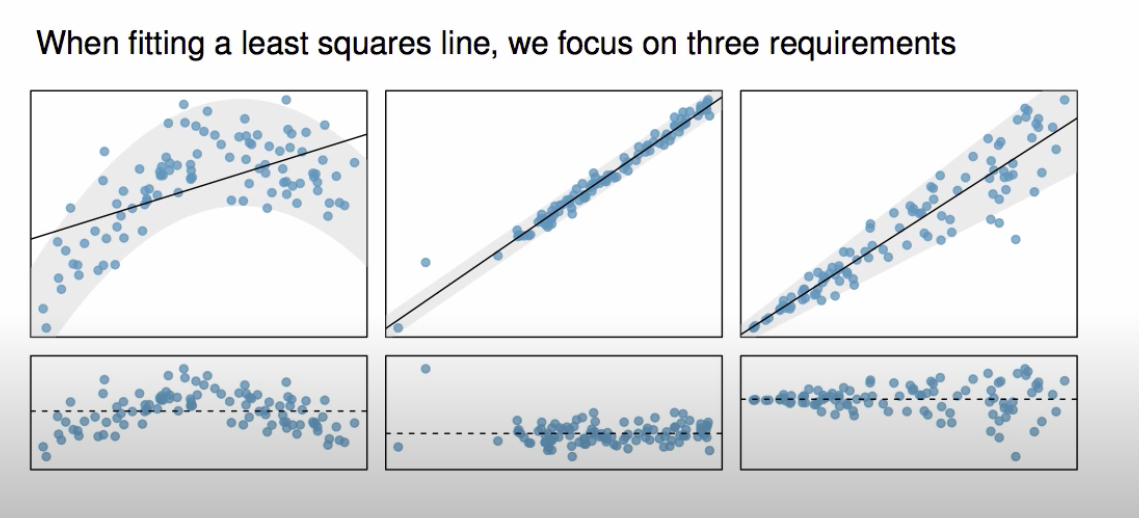
• Conditions for using least squares regression:
  • The Data should show a linear trend:
    • If not, another method should be used.
  • The residuals should be normally distributed:
    • If not, the results may not be reliable as there are lots of outliers and influential points.
  • Constant variability of residuals:
    • The variability of the residuals should be constant across all values of the explanatory variable.
• The image below show errors in the least squares conditions:
  • 
  • First: image shows non-linear trend, as data trends upwards and then downwards later.
  • Middle: image shows non-normal residuals, notice the big outlier and points are empty towards the left.
  • Last: image shows non-constant variability, as the variability of the residuals fan our as the explanatory variable increases.
• We don’t know how the data outside of our limited window behaves, so we can’t make predictions outside of the window.
• Linear regression indicates a relationship but not causation.

Types of outliers in linear regression ⁵

• Outliers are observations that fall out of the cloud of points.
• Some outliers are influential points that have a large effect on the slope of the regression line.
• Points that fall horizontally away from the cloud of points tend to pull harder on the line so we call them high leverage points.
• If one of those high leverage points actually invokes its influence on the slope of the line, we call it an influential point.
• Don’t remove outliers without a good reason.

How to do simple linear regression in JASP (14-7) ⁶

• Correlation = regression with two variables.
• Load the data into JASP.
• Plot the data to check for conditions:
  • Use Regression > Classical > Correlation from the top menu.
  • Load the x variable (predictor, explanatory) first and then the y variable (response).
  • Select Display Pairwise under Additional Options.
  • Under Plots, select Scatterplot; which allows as to check linearity, outliers, and influential points.
  • Under Plots, select Densities for variables to check for normality.
  • You can use the Assumption Checks to check for the assumptions of linear regression.
• Do the Regression analysis:
  • Use Regression > Classical > Linear Regression from the top menu.
  • Dependent variable is the y variable.
  • Covariate is the x variable.
  • Set the Method to Enter.
  • Under Statistics:
    • Select Regression Coefficient > Confidence intervals.
    • Select Regression Coefficient > Descriptives.
    • Select Residuals > Statistics to check for outliers and influential points (Std. Residuals should be between -3 and 3).
    • Select Residuals > Durbin-Watson to check for independence of observations (Durbin-Watson statistic should be between 1 - 3).
  • Under Plots:
    • Select Residuals plots > Residuals vs Histogram to check for normality.
    • Select Q-Q plot standardized residuals to check for normality.
    • Select Residuals vs predicted to check for homoscedasticity.

References

---

1. Diez, D. M., Barr, C. D., & Çetinkaya-Rundel, M. (2019). Openintro statistics - Fourth edition. Open Textbook Library. https://www.biostat.jhsph.edu/~iruczins/teaching/books/2019.openintro.statistics.pdf Read Chapter 8- Introduction to linear regression
   Section 8.1 - Fitting a line, residuals, and correlation from page 305 to 316 Section 8.2 - Least squares regression from page 317 to 327 Section 8.3 - Types of outliers in linear regression from page 328 to 330 ↩

2. Goss-Sampson, M. A. (2022). Statistical analysis in JASP: A guide for students (5^th ed., JASP v0.16.1 2022). https://jasp-stats.org/wp-content/uploads/2022/04/Statistical-Analysis-in-JASP-A-Students-Guide-v16.pdf Read Descriptive Statistics (pp. 14- pp. 27) Read ANOVA (pp. 91- pp. 98) Read Correlation Analysis, Running correlation from page 67 to 70
   Read Regression from page 73 to 78 ↩

3. OpenIntroOrg. (2014a, January 26). Line fitting, residuals, and correlation [Video]. YouTube. https://youtu.be/mPvtZhdPBhQ ↩

4. OpenIntroOrg. (2014b, January 27). Fitting a line with least squares regression [Video]. YouTube. https://youtu.be/z8DmwG2G4Qc ↩

5. OpenIntroOrg. (2014c, February 11). Types of outliers in linear regression [Video]. YouTube. https://youtu.be/jZEKAlo1E54 ↩

6. Research By Design. (2020, June 5). How to do simple linear regression in JASP (14-7) [Video]. YouTube. https://youtu.be/vKGphOrzze8 ↩