6. Measuring Total Output and Income & Aggregate Demand and Aggregate Supply
Measuring Total Output and Income 1
Limitations of GDP 2
- GDP (Y) is the some of:
- Consumption (C).
- Investment (I).
- Government spending (G).
- Net exports (NX).
- GDP = C + I + G + NX or Y = C + I + G + NX
- GDP per capita: GDP divided by the population of a country.
- GDP per capita is a useful measure of the standard of living or well-being of the average person in a country.
- GDP: the aggregate measure of total production in an economy in a given period.
- GDP is useful for Measuring:
- Economic activity.
- Size or influence of an economy.
- GDP is not useful for:
- It does not include non-market activities, that is, activities that are not exchanged for money; such as taking care of your children vs hiring a babysitter.
- It does include under-the-table transactions, that is, transactions that are not reported to the government for tax purposes or because they are illegal.
- It does not include information about pollution, that is, polluting the world toady will affect economic activity in the future.
- Other things, like health, happiness, stress, feeling of community, etc; are not included in GDP.
- It does not include the distribution of income and inequality.
Circular Flow of Income and Expenditures 3

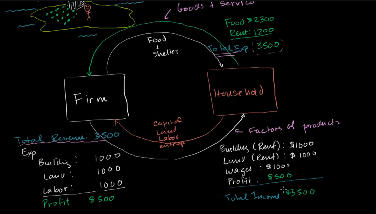
- The household sector is the group of people who live in the same house and share income and expenses.
- Households supply firms with factors of production, such as labor, land, and capital. Firms pay households for these factors of production, and sell them goods and services.
- Households has total expenditures, firms have total revenue, and households again have total income.
- If the 3 numbers included in the GDP, then we are tripping the GDP.
- Only one number should be included in the GDP, which is the total income of the households.
Aggregate Demand and Aggregate Supply 4
Aggregate Demand 5
- Aggregate demand and supply are a macroeconomic model that works on the economy as a whole.
- Axis:
- X-axis: Real GDP, the total quantity of goods and services produced in the economy.
- Y-axis: Price level, the average price of goods and services in the economy.
- Aggregate demand curve:
- It is downward sloping.
- Ceteris paribus, as the price level increases, the quantity of goods and services demanded decreases.
- Ceteris paribus, as the price level decreases, the quantity of goods and services demanded increases.
- If prices are high, GDP will shrink.
- If prices are low, GDP will grow.
- Causes of the downward slope of the aggregate demand curve:
- Wealth effect:
- As prices decrease, the real value of money increases, and people feel wealthier, so they spend more.
- If people have the same money, but prices decrease, they will feel wealthier as they can buy more with the same money.
- If prices increase, people can buy less with the same money, so they feel poorer, and demand less.
- Interest rate effect:
- As prices decrease, interest rates decrease, so people borrow more and spend more.
- Sometimes, the interest rate is fixed, so the price level will not affect the interest rate.
- Sometimes, it is called the Saving effect.
- If prices go down:
- People will spend less money on essentials, and save more.
- More saving means more money in the banks.
- More money in the banks increases the supply of money, so the interest rate decreases (the price of borrowing money decreases).
- The lower interest rate encourages people to borrow more money and spend more.
- More money to spend means more demand and more investment.
- More investment means more production, and more jobs, and more GDP.
- If prices go up:
- People will spend more money on essentials, and save less.
- Less saving means less money in the banks, so the interest rate increases.
- The higher interest rate discourages people to borrow money and spend less.
- Exchange rate effect:
- As prices decrease, the currency depreciates, so exports increase, and imports decrease.
- If prices go down:
- Interest rates go down, so people will find it more profitable to save money in other countries, where interest rates are higher.
- People will sell their currency and buy other currencies, so the value of the currency will decrease.
- Goods and services will become cheaper for customers in other countries (as other currencies convert to more of the local currency).
- Foreign countries will demand more goods and services from the local country, and exports will increase.
- To accommodate the increase in exports, local companies will increase production, and GDP will increase.
- If prices go up:
- Interest rates go up, more people converting to local currency as it gets stronger.
- Stronger currency means that goods are more expensive for customers in other countries.
- LEss demand from other countries, so exports will decrease, and GDP will decrease.
- Wealth effect:
- Aggregate Demand shifters:
- Anything affecting C, I, G, and NX.
- Example: C: Consumer spending:
- Tax cuts: tax cuts make people feel wealthier, so they spend more, and consumption increases.
- Tax increases: tax increases make people feel poorer, so they spend less, and consumption decreases.
| Aspect | Demand | Aggregate Demand |
|---|---|---|
| Level | Micro economic | Macro economic |
| Axis X | Quantity | Real GDP |
| Axis Y | Price | Price level |
| Representation | One product market | All products, or the entire economy |
| Slope | Downward | Downward |
| Causes of downward slope | Substitution effect, income effect | Wealth effect, interest rate effect, exchange rate effect |
| Demand shifters | consumer preferences, prices of related goods, income, demographics, and buyer expectations. | Anything affecting C, I, G, and NX (see above). |
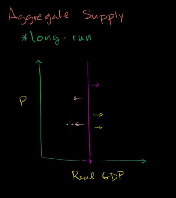
Long-run Aggregate Supply 6
- Time for a lot of fixed costs and fixed prices to adjust, change, or expire.
- Aggregate supply in long term is vertical, that is, it does not depend on the price level.
- Shifters of the long-run aggregate supply curve:
- Population increase: more people, more labor, more production => more GDP.
- Technology advancements: more technology, more production => more GDP.
- Resource availability: more resources discovered, more production => more GDP.
- Low unemployment: more people working, more production => more GDP.
- War: population decrease or factories destroyed, less production => less GDP.

Short-run Aggregate Supply 7
- In the short run, the aggregate supply curve is upward sloping.
- Causes of the upward slope of the short-run aggregate supply curve:
- Misperception theory:
- Firms may think that the price increase is due to an increase in demand for their product, so they produce more.
- Misunderstanding the price increase as an increase in demand, as in microeconomics.
- According to the microeconomic’s law of supply, if the price increases, the quantity supplied increases.
- Sticky wages, costs, prices theory:
- Wages are sticky, that is, they do not change quickly.
- Not all prices move at the same time, some move faster than others.
- Sickness may be due to contracts, unions, menu costs, or other reasons.
- If prices increase, while wages are still sticky, firms will interpret the increase in profits as an increase in demand, so they will produce more.
- In the long run, wages will adjust, and prices will adjust, and the temporal profit will disappear.
- Misperception theory:
Short-run and Long-run Equilibrium and the Business Cycle 8
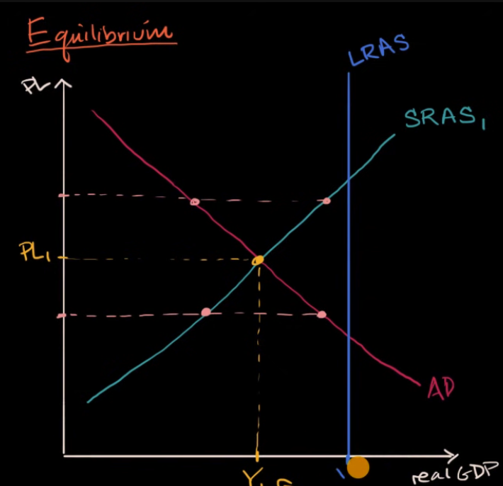
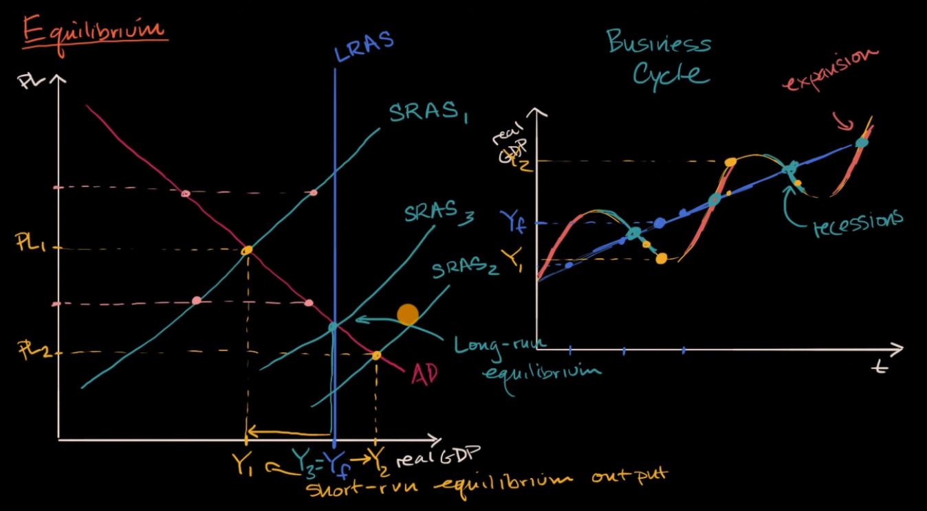
- Short run equilibrium:
- The intersection of the aggregate demand curve and the short-run aggregate supply curve.
- The price level and the real GDP are determined by the intersection of the two curves.

- Long run equilibrium:
- The intersection of the aggregate demand curve and the long-run aggregate supply curve.

References
-
Rittenberg, L. & Tregarthen, T. (2009). Principles of Economics. Flat World Knowledge. Chapter 21: Measuring Total Output and Income.https://my.uopeople.edu/pluginfile.php/1894561/mod_book/chapter/527815/Principles%20Of%20Economics%20Chapter%2021.pdf ↩
-
Khan Academy. (2018, February 5). Limitations of GDP | Economic indicators and the business cycle | AP Macroeconomics | Khan Academy [Video]. Youtube. https://youtu.be/SXMhCO2vYcE ↩
-
Khan Academy. (2012, February 1). Circular flow of income and expenditures | Macroeconomics | Khan Academy [Video]. Youtube. https://youtu.be/Hfz1bwK5C4o ↩
-
Rittenberg, L. & Tregarthen, T. (2009). Principles of Economics. Flat World Knowledge. Chapter 22: Aggregate Demand and Aggregate Supply. https://my.uopeople.edu/pluginfile.php/1894566/mod_book/chapter/527823/Principles%20Of%20Economics%20Chapter%2022.pdf ↩
-
Khan Academy. (2012, March 1). Aggregate demand | Aggregate demand and aggregate supply | Macroeconomics | Khan Academy [Video]. YouTube. https://yougttu.be/oLhohwfwf_U ↩
-
Khan Academy. (2jtg,jjű012, March 2). Long-run aggregate supply | Aggregate demand and aggregate supply | Macroeconomics | Khan Academy [Video]. YouTube.https://youtu.be/8W0iZk8Yxhs ↩
-
Khan Academy. (2012, March 5). Short run aggregate supply | Aggregate demand and aggregate supply | Macroeconomics | Khan Academy [Video]. YouTube. https://youtu.be/3nbalsyibKU ↩
-
Khan Academy. (2018, February 23). Short run and long run equilibrium and the business cycle | AP Macroeconomics | Khan Academy [Video]. YouTube. https://youtu.be/dD_9KBz3pN0 ↩