7. Ranking in a Complete Search System
7.1 Efficient scoring and ranking 1
- 7.1.1 Inexact top K document retrieval:
- Retrieve K documents whose scores are very close to those of the K best.
- While avoiding computing scores for most of the N documents in the collection.
- 7.1.2 Index elimination:
- For a query with multiple terms, we consider documents that at least contain one of the query terms; and then:
- Consider only documents with IDF passing a certain threshold => low IDS documents are ignored => fewer posting lists to retrieve and process.
- Only consider documents that contain a certain fraction of the query terms => E.g. Ignore documents that contain less than 3 terms (in a query of 5 terms) => fewer documents to consider.
- Both thresholds are highly application-dependent, and a problem may arise if we choose thresholds that return less than K documents, where we can not the required K number of documents.
- For a query with multiple terms, we consider documents that at least contain one of the query terms; and then:
- 7.1.3 Champion lists:
- Also known as fancy lists or top docs.
- For each term, we store a list of documents that have the highest scores for that term.
- When a query is issued, we only consider documents in the champion lists.
- Champion lists are usually small (e.g. 1000 documents) and can be stored in memory.
- Champion lists can be precomputed offline.
- The length of the champion list r is a parameter that can be tuned, but it is determined while indexing and before the query is issued.
- The number of documents to return k depends on the query itself and is determined at query time.
- Problem: if we choose r that is smaller than k, we may not be able to retrieve the top k documents.
- 7.1.4 Static quality scores and ordering:
- This improves the selection of champion lists.
- Static quality scores are query-independent scores that measure the quality of a document.
- Net score of a document = static quality score + dynamic score (computed at query time) = static score + cosine similarity.
- \(\text{net-score(q,d)} = g(d) + \frac{\vec{d} \cdot \vec{q}}{\|\vec{d}\| \|\vec{q}\|}\)
- Where \(g(d)\) is the static quality score of document \(d\) and its value is between 0 and 1.
- The net score now is between 0 and 2 (0-1 static score + 0-1 cosine similarity).
- We may also store a second champion list containing r documents right below the first champion list.
- When the query is issued; if the first champion list returns less than k documents, we can use the second champion list to retrieve the remaining documents.
- 7.1.5 Impact ordering:
- The idea is to order the documents based on a key that is different from the term ID.
- Instead, terms are ordered by their tf(t,d) (term frequency in the document).
- Then, we don’t need to process all items in a champion list; but only until we reach the k documents or the tf(t,d) drops below a certain threshold.
- Another idea is to order the terms by their IDF.
- 7.1.6 Cluster pruning:
- A preprocessing step that clusters documents into groups.
- At query time, only a few clusters are considered:
- Pick N^½ documents randomly that are closest to the query, and call them leaders.
- For each document that is not a leader, compute its nearest leader.
- Not leader documents are called followers.
- The process also accepts two parameters b1, and b2 which control the number of leaders and followers.
- The randomness is proven to be effective in practice.
7.2 Components of an information retrieval system 1
- 7.2.1 Tiered indexes:
- We store the index in multiple tiers, where each tier is a different index.
- We always start from tier 1, and we only process the next tier if we do not reach the required k number of documents.
- E.g.: tier 1 contains all words with tf(t,t) > 20, and tier 2 contains all words with 20 > tf(t,t) > 10; and so on.
- 7.2.2 Query-term proximity:
- We can use the position of the query terms in the document to improve the ranking.
- The window w (number of words) in the document that contains all query terms.
- Documents with smaller windows are ranked higher.
- E.g.: if the query is “Ahmad student”:
- Document 1:
Ahmad is a student at the University of Jordan. Window = 3. - Document 2:
Ahmad is a web developer, he used to be a student. Window = 8. - Document 1 is ranked higher than Document 2, as it has a smaller window that contains all query terms.
- Document 1:
- 7.2.3 Designing parsing and scoring functions:
- This depends on user population, query distribution, and the collection of documents itself.
- Query parser:
- It is a function that translates a user query into a query that can be processed by the search engine; that is, adding/removing the necessary operators and terms.
- Sometimes, more than one query is generated by the query parser for each user query, all of them are processed and the results are merged.
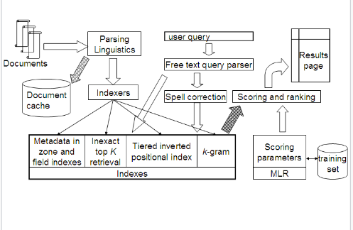
- 7.2.4 Put it all together:
- We have now studied all the components necessary for a basic search system that supports free text queries as well as Boolean, zone and field queries.

7.3 Vector space scoring and query operator interaction 1
- It helps answer boolean, wildcard, and phrase queries.
References
-
Manning, C.D., Raghaven, P., & Schütze, H. (2009). An Introduction to Information Retrieval (Online ed.). Cambridge, MA: Cambridge University Press. Chapter 7: Computing Scores in a Complete Search System. http://nlp.stanford.edu/IR-book/pdf/07system.pdf ↩↩↩