8. Searching and Indexing
9. searching 1
- Searching is:
- The process to determine if an element within a particular value is a member of a particular set.
- An attempt to find the record within a collection of records that has a particular key value (exact match query).
- Finding all records in a collection whose key value satisfies a particular condition (criteria) (range query).
- Searching algorithms categories:
- Sequential search and list methods.
- Direct access by key value (hashing).
- Tree indexing methods.
9.1 Searching Arrays
Jump Searchis an algorithm used for searching; steps:- Sort the array.
- Define the jump size (j), which is the number of elements to be skipped in each jump; the best value is
sqrt(n)where n is the size of the array. - Start from the first element, compare it with the key value, if it is less than the key value, jump to the next element by adding the jump size to the current index. like:
for (int i = 0; i < n; i += j). - If the current element (jumped to at
i = m*j) is greater than the key value, then the target element is somewhere betweeni-jandi, so we do a linear search in this range. - We take a separate list from
i-jtoiand do a linear search on it (sequential search). - If the key value is not found, then it is not in the array.
Binary SearchThe generalization of the jump search where the jump size is ½ of the array size.Dictionary Searchorinterpolation searchis a special variation of the Binary search where we know more details about the distribution of the keys we can make better compute jump sizes where the initial jump size (j) can be computed asj = (key - L[0])/ L[n] - L[0]assuming the list is sorted andkeyis the key value we are searching for, andL[0], L[n]are the first and last elements keys of the list respectively, for the next jump we use the same formula but with the sublist we are currently in.Quadratic Binary Search (QBS)is a variation of the dictionary search, Where after the first jump, we use a different way to compute the jump size within the sublist and so on for the next sublists until the element is found or not found. The time complexity for QSB isO(log(log(n)))which is better than theO(log(n))for the dictionary search.
9.2 Self-Organizing Lists
- Ordering the list elements can be done on:
- Keys: elements are ordered by their key values.
- Access Frequency: Elements with higher expected access frequency are placed at the beginning of the list which improves the sequential search speed.
- The 80/20 rule is an example of a
Zipf distributionwhere 20% of the elements are accessed 80% of the time and it appears a lot in practice. - This is potentially a useful observation that typical “real-life” distributions of record accesses, if the records were ordered by frequency, would require that we visit on average only 10-15% of the list when doing sequential search.
- The problem is that access patterns change, and what was once a high-frequency item may become a low-frequency item.
- Self-organizing lists:
- Modify the order of records within the list based on the actual pattern of record access rather than on the expected pattern of access.
- They adapt to changes in the access pattern.
- They have heuristics to govern the
reorderingof the list that are similar to the buffer-pool:FIFO,LRU,LFU,MFU.
- Self-Organizing Lists Heuristics:
- Count:
- Count the times each item is accessed and maintain the list ordered according to this count.
- Similar to
Least Frequently Used (LFU)where the items with lower counts are placed at theendof the list. - When item is accessed its count is incremented and the list is reordered moving the item
forwardin the list. - The count does not react to the changing of access patterns overtime, once an element is accessed enough number of times it will stay in the front event if it is not accessed anymore.
- Move to Front (MTF)
- Every time an item is accessed, it is moved to the front of the list pushing the other items back.
- Similar to
Least Recently Used (LRU)where the items that are accessed recently are placed at thefrontof the list. - This easy for List implementation but it is not efficient for Array implementation as it requires shifting the elements.
- The MTF responds well to the local changes in frequency of access as the element will be at the front during the period of high access frequency and will be moved back when the access frequency decreases.
- MTF does badly if elements are accesses in a cyclic pattern (repetitive sequence of accesses) e.g.
1,2,3,4,5, 1,2,3,4,5, 1,2,3,4,5as the elements will be moved back and forth (the numbers correspond to the index of the element in the list).
- Transpose
- Swap the accessed element with the element before it.
- Good for both list and array implementations.
- Elements that are accessed frequently will
tend to slowly movetoward the front of the list, and thenslowlymove back toward the end of the list when they are no longer accessed.
- Count:
- Advantages of Self Organizing Lists:
- No need to sort the list or maintain a sorted list, which makes the insertions and deletions faster.
- Simpler to implement than the search trees; and more suitable for smaller lists.
- No need for additional storage space.
- For applications that already coded; the code changes are minimal to transform a normal list to a self-organizing list.
9.3 BitMaps
- Bit Vectors for Representing Sets = BitMaps.
- Bit Vector (Bit map) is a data structure that represents a set of elements as a vector of bits, where each bit represents an element in the set, to check if the element is in the original set we check the corresponding bit in the vector.
- Example:
- To represent
[0, 1, 10, 50]we create a bit vector of size 51 (the largest element in the set) and set the bits at the corresponding indices to 1. like:[1, 1, 0, 0, 0, 0, 0, 0, 0, 0, 1, 0, ...] - where 1 indicates that element is in the set and 0 indicates that the element is not in the set.
- To search for the item
10we check the bet vector at index10and if it is 1 then the element is in the set, or if it is 0 then the element is not in the set. - To insert an element
20we have to do 2 things: 1. actually insert the element in the original list. 2. set the bit at index20to 1.
- To represent
9.4 Hashing
- Hashing used in the direct access based on the key value searching, where finding a record starts by doing some computations to calculate the position of the record in the list, where the items are already sorted according to the same computation.
- Hashing makes some operations harder:
- Hashing is not good where multiple records with the same key are allowed.
- Hashing is not good for range queries.
- We cannot find all records with keys falling in a given range.
- We cannot find the smallest or largest key in the list.
- We cannot visit records in order according to their key values.
- Hashing is most appropriate for exact-match queries where we are looking for a record with a given key value.
- Hashing is suitable for both in-memory and disk-based searching and is one of the two most widely used methods for organizing large databases stored on disk (the other is the B-tree).
- Terminology:
- Slot: a position within the hash table that may hold a record (s), usually represented by an array.
- Hash function: a function that maps the key value to the slot index.
- Collision: when two records have the same hash value and are mapped to the same slot.
- Collision resolution policy: the process of handling collisions to find the individual record within the slot.
- Hashing generally takes records whose key values come from a large range and stores those records in a table with a relatively small number of slots.
- The Collision resolution policies is divided into two classes:
- Open Hashing or Separate Chaining: each slot in the hash table is a head of a linked list, and all records that hash to the same slot are placed in the linked list.
- Closed Hashing or Open Addressing: all records are stored in the hash table itself, and when a collision occurs, another slot in the hash table is chosen to store the record.
9.4.1 Hash Functions
- Perfect Hashing: a hash function that maps each key to a unique slot, so there are no collisions.
- Characteristics of a good hash function:
- Efficiency: the hash function should be easy to compute.
- Uniformity: distributes they hashed keys so that every slot has equal probability of being filled = the hash function should distribute the keys uniformly across the slots, regardless of the distribution of the keys themselves.
- Dependability: the hash function should depend only on the key value and not on the number of slots in the table.
- There are many reasons why data values might be poorly distributed:
- Natural frequency distribution of the data: where a few of the entities occur very frequently and most of the entities occur very rarely.
- Collected data are likely to be skewed due to factors like rounding, truncation, or other data collection errors.
- If the input is text, the distribution of the first letter of the words is poorly distributed (e.g. the letter
eis more frequent than the letterz).
- When designing a hash function:
- If we know the distribution of the keys, the hashing function should be distribution-dependent that avoids assigning high number of keys to the same slot. e.g. if we are hashing the first letter of the words, the hashing function should not use a slot for each first letter as the letter
eis more frequent than the letterz. - If we don’t know anything about the frequency of the keys; the hashing function should be distribution-independent that distributes the keys uniformly (evenly) across the slots.
- If we know the distribution of the keys, the hashing function should be distribution-dependent that avoids assigning high number of keys to the same slot. e.g. if we are hashing the first letter of the words, the hashing function should not use a slot for each first letter as the letter
-
Examples of hashing functions:
- Hash integers in
mslot hash table:- use
h(int k) = k%mwheremis the number of slots in the hash table. - E.g. if
m=10thenh(1234) = 1234%10 = 4. - This function distributes the keys poorly, as it relies on the most significant digits of the key value, which are often poorly distributed.
- use
- Mid-Square method:
- Square the key value and extract the middle
rbits as the hash value. - E.g. if the key is
1234andr=4thenh(1234) = 1234^2 = 1522756 = 101110111011110011100and the middle 4 bits are1110soh(1234) = 14. - This function distributes better as we no longer relying on the distribution of one digit in the key value.
- Square the key value and extract the middle
- Sum the ASCII values of chars in a string
- Each ASCII letter in a string correspond to integer, e.g,
ais97,bis98,cis99, etc. - To hash a string, we sum the ASCII values of the chars in the string, resulting in an integer, then we use the integer as the hash value.
- E.g.
h("abc") = 97+98+99 = 294. - An example of Folding approach, where we divide the key into several parts, sum the parts, and then use the sum as the hash value.
- The computed hash is independent of the order or characters in the string, that is
h("abc") = h("cba") = h("bca") = 294. - This function poorly distributes the keys, as the sum of
nASCII values will fall within the range97nto122n, which is a small range compared to the range of the hash table (e.g. ifm=1000then the range is0to999, then only ranges between 650 and 900 will be filled).
- Each ASCII letter in a string correspond to integer, e.g,
-
sFold:
- This function takes a string as input. It processes the string four bytes at a time, and interprets each of the four-byte chunks as a single long integer value. The integer values for the four-byte chunks are added together.
- In the end, the resulting sum is converted to the range 0 to M − 1 using the modulus operator.
- E.g.
sFold('aaaabbbb') = fSum('aaaa') + fSum('bbbb') = 1633771872 + 1633771872 = 3267543744 = 3267543744%101 = 75. The hash value is75assuming thatM=101so the we have 101 slots in the hash table.
long sfold(String s, int M) {
    int intLength = s.length() / 4;
    long sum = 0;
    for (int j = 0; j < intLength; j++) {
        char c[] = s.substring(j*4,(j*4)+4).toCharArray();
        long mult = 1;
        for (int k = 0; k < c.length; k++) {
            sum += c[k] * mult;
            mult *= 256;
        }
    }

    char c[] = s.substring(intLength * 4).toCharArray();
    long mult = 1;
    for (int k = 0; k < c.length; k++) {
        sum += c[k] * mult;
        mult *= 256;
    }

    return(Math.abs(sum) % M); // modula M
}
- Hash integers in
9.4.2 Open Hashing
- Open Hashing or Separate Chaining: each slot in the hash table is a head of a linked list, and all records that hash to the same slot are placed in the linked list.
- The items within each slot (linked list) are sorted in different ways: insertion order, key value order, or by frequency of access order.
- Open hashing is suitable when keeping the HT in memory, as the linked lists are easy to manipulate.
- Using open hashing for in disk HT is not efficient, as the linked lists are not easy to manipulate in disk (items may be scattered in different locations in the disk resulting in multiple disk accesses to retrieve the items).
- Open hashing is similar to BinSort as each slot can be thought as a bin.
9.4.3 Closed Hashing
- Closed Hashing or Open Addressing: all records are stored in the hash table itself, each Record has a home position
hp = h(k). - When the
hpslot already occupied, the resolution collision policy determines a different slot to place the record, and if this also occupied, the policy determines another slot, and so on (recursively) until an empty slot is found. - When looking for item, the home position is computed, then the collision policy traverse next possible slots until the item is found or an empty slot is found (meaning the item is not in the hash table).
- Popular closed hashing implementations:
- Linear Probing
- Bucket Hashing
Bucket Hashing
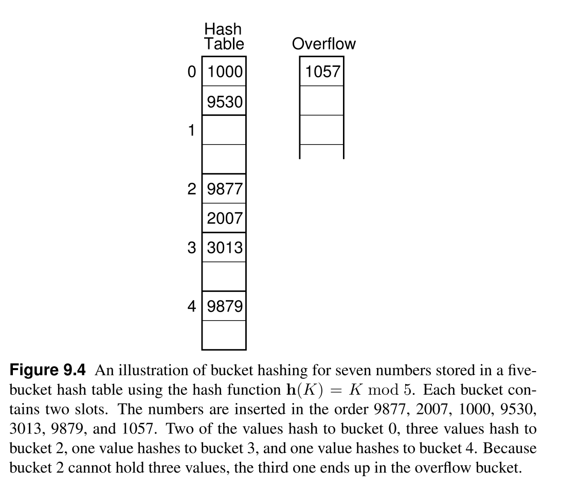
- An implementation of closed hashing where the slots are grouped into buckets. A HT with M slots is divided into B buckets, each bucket has
M/Bslots. - The hash function assigns records to the first slot within a bucket, and if it is occupied, the bucket is sequentially searched for an empty slot.
- If all slots within a bucket are occupied, the new item is placed in the
overflow bucket. - The
overflow bucketis a special bucket that has infinite capacity at the end of the hash table. - A variation of the bucket hashing adjust the borders of buckets as needed (taking from the slots assigned to the next bucket), so that it only uses the overflow bucket when all slots in the hash table are occupied or if both this bucket and the next bucket are full.
- Bucket hashing is good for implementing in-disk hash tables as the size of the bucket can be set to the size of the disk block, and then the entire block (bucket) can be read to memory at once reducing the number of disk accesses.
Linear Probing
- An implementation of closed hashing that has no bucketing and a collision resolution policy that uses any possible slot in the hash table.
- The hash function generates a sequence of slots to place the record, and when looking for a record, the same sequence is used to search for the record.
- When inserting a new record, the sequence of slots is searched until an empty slot is found, and the record is placed in the empty slot.
- The sequence of slots is called
probe sequenceand is generated bt aprobe functionwe denote it asp(k,i)wherekis the key value andiis the probe number. - To avoid infinite searching loops, the table must keep track of the number os stored records and refuse to insert a table that has one free slot.
- This is one of the worst collision resolution policies as it causes clustering.
- Primary Clustering: as items have equal probability of being placed in any slot initially, after a few insertions, the probabilities will change and some slots will have higher probability of being filled than others, making items to cluster in these slots.
Improved Collision Resolution Methods
- Improvement 1: move by constant c > 1 when probing:
- One improvement is to use the linear probing, but move the items down using a constant c that is different than 1 causing the records with adjacent home positions to be placed in different slots.
- Constant c must be relatively prime to M to generate a linear probing sequence that visits all slots in the table (that is, c and M must share no factors) where M is the size of the hash table (number of slots).
- This method does not stop clustering, but it reduces it.
- Improvement 2: Pseudo-random probing:
- The perfect probing function that choses a random slot for inserting the next element, but this is not possible because we have to generate the same sequence when looking for the item.
- When creating a hash table, we can generate a random permutation of the slots and use this permutation as the probe sequence.
- When looking for an item, we use the same permutation to search for the item that was used to insert the item.
- This method eliminates clustering as the items are placed in random slots.
- Improvement 3: Quadratic probing:
- The probe sequence is generated by a quadratic function
p(k,i) = (h(k) + c1*i^2 + c2*i + c3) mod Mwherec1, c2, c3are constants andiis the home position. - Thus, if the table is less than half full, we can be certain that a free slot will be found
- The probe sequence is generated by a quadratic function
9.4.4 Analysis of Closed Hashing
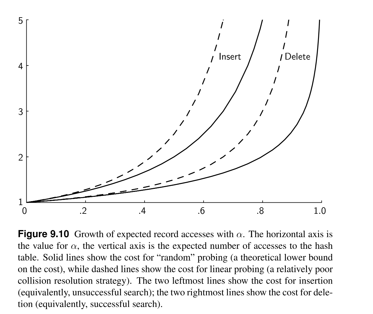
- Load Factor: the ratio of the number of records in the table to the number of slots in the table (a = N/M) where N is the number of current records and M is the size of the table.
- The rule of thumb is to design a hashing system so that the hash table never gets above half full. Beyond that point performance will degrade rapidly.
- Thus, the more space available for the hash table, the more efficient hashing should be.
- Deleting a record:
- Deleting a record must not be done simply by nulling the record, as this will cause the search to stop when it reaches the null record before continuing the probe sequence.
- Instead, the value is kept but the record is marked as deleted and so it is available for the next insertion.
- Per diagram below, the more a is, the more the number of accesses to find an item increases; so that when the table is nearly empty (a is small) the number of accesses is almost 1.
10. Indexing 2
- Entry-sequenced files:
- An entry-sequenced file stores records in the order that they were added to the file.
- The disk-based equivalent to an unsorted list.
- they do not support efficient search.
- Indexing:
- Indexing is the process of associating a key with the location of a corresponding data record.
- The index file could be sorted or organized as tree, thus imposing logical order on the records without physically rearranging them.
- Terminology:
- Primary Key: is the unique key that identifies a record, usually unsuitable for searching as it is not descriptive.
- Secondary Key: is a property on the records that is used for searching, usually descriptive; it is not unique and may not be present in all records.
- Secondary Key index: or simply Secondary Index will associate a secondary key with its primary key (thus, the location of the record) for each record that has the secondary key value.
- Primary Index: is an index that associates the primary key with the location of the record on disk.
- Usually, only the primary keys points to the location of the record on disk, while every secondary index points to the primary key itself.
- B-trees are the most widely used indexing method for large disk-based databases, and for implementing file systems.
10.1 Linear Indexing
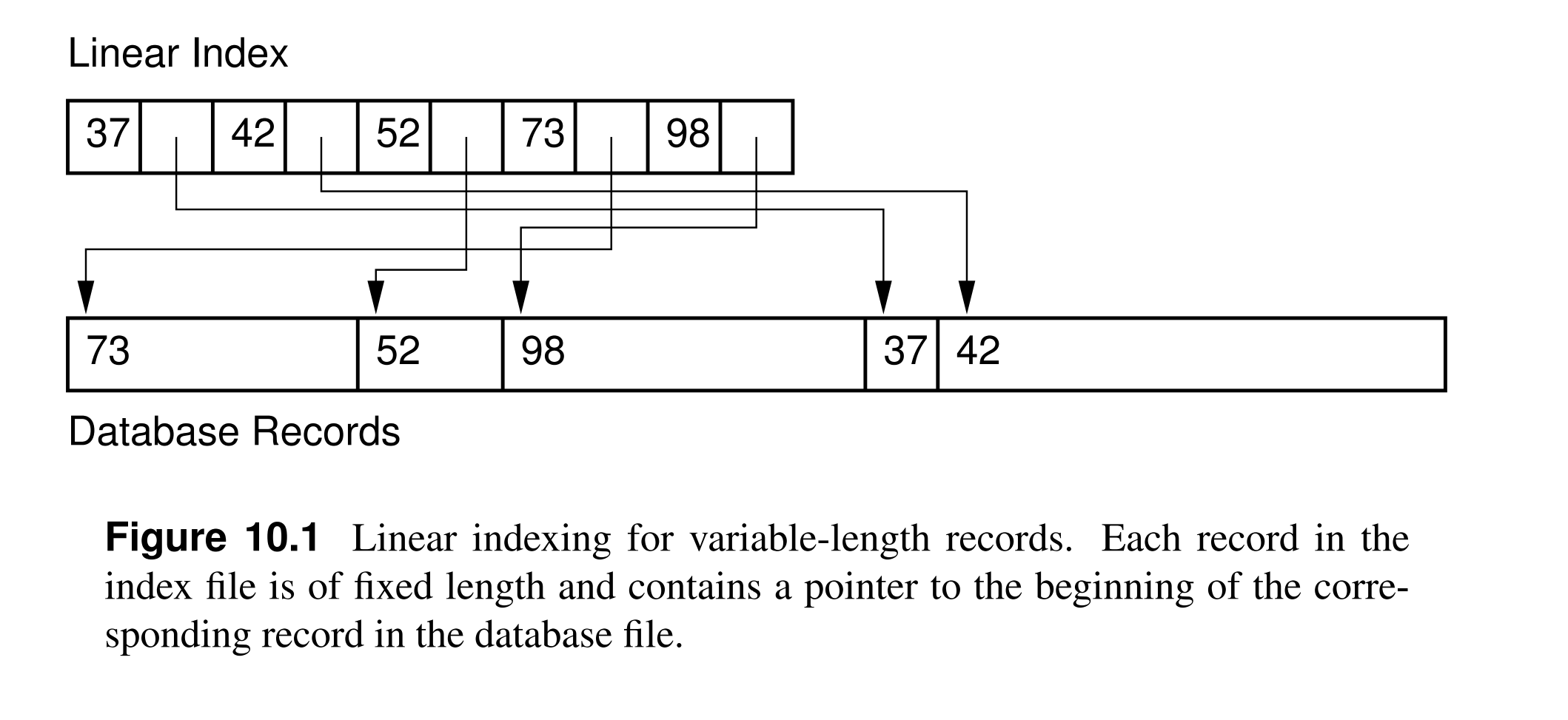
- A linear index is an index file organized as a sequence of key/pointer pairs where the keys are in sorted order and the pointers either:
- Point to position of the complete record on disk.
- Point to the position of the primary key on the primary index.
- Hold the actual value of the primary key.
- Advantages of Linear index:
- Allows for efficient search and random access to database records, because it is amenable to binary search.
- It simplifies access to variable-length records as the index holds only fixed-length keys and pointers.
- The linear index can be stored in memory or on disk, if it does not fit in memory.
Two level linear index
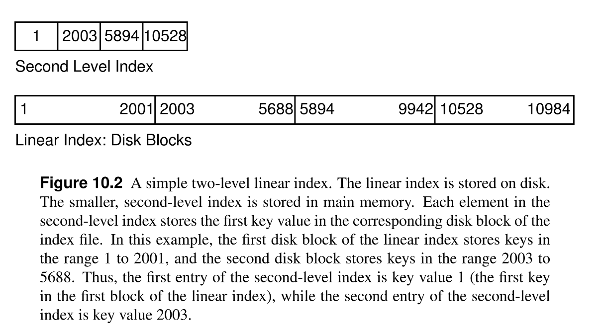
- Searching in on-disk linear index is expensive as multiple disk accesses are required.
- The solution to use another in-memory index that maps the pages of the on-disk index and their key ranges to the disk addresses of the pages.
- Searching for a record > the in-memory index determine which disk block (from the on-disk index) contains the record > the disk block is read into memory > the record is searched for in the block > another disk access is required to read the actual record.
- Every Search requires at least 2 disk accesses (one for the index and one for the record).
Sorted Two-Dimensional Array index
- Secondary keys are not unique, so that repeating the same value in the index is a waste of space.
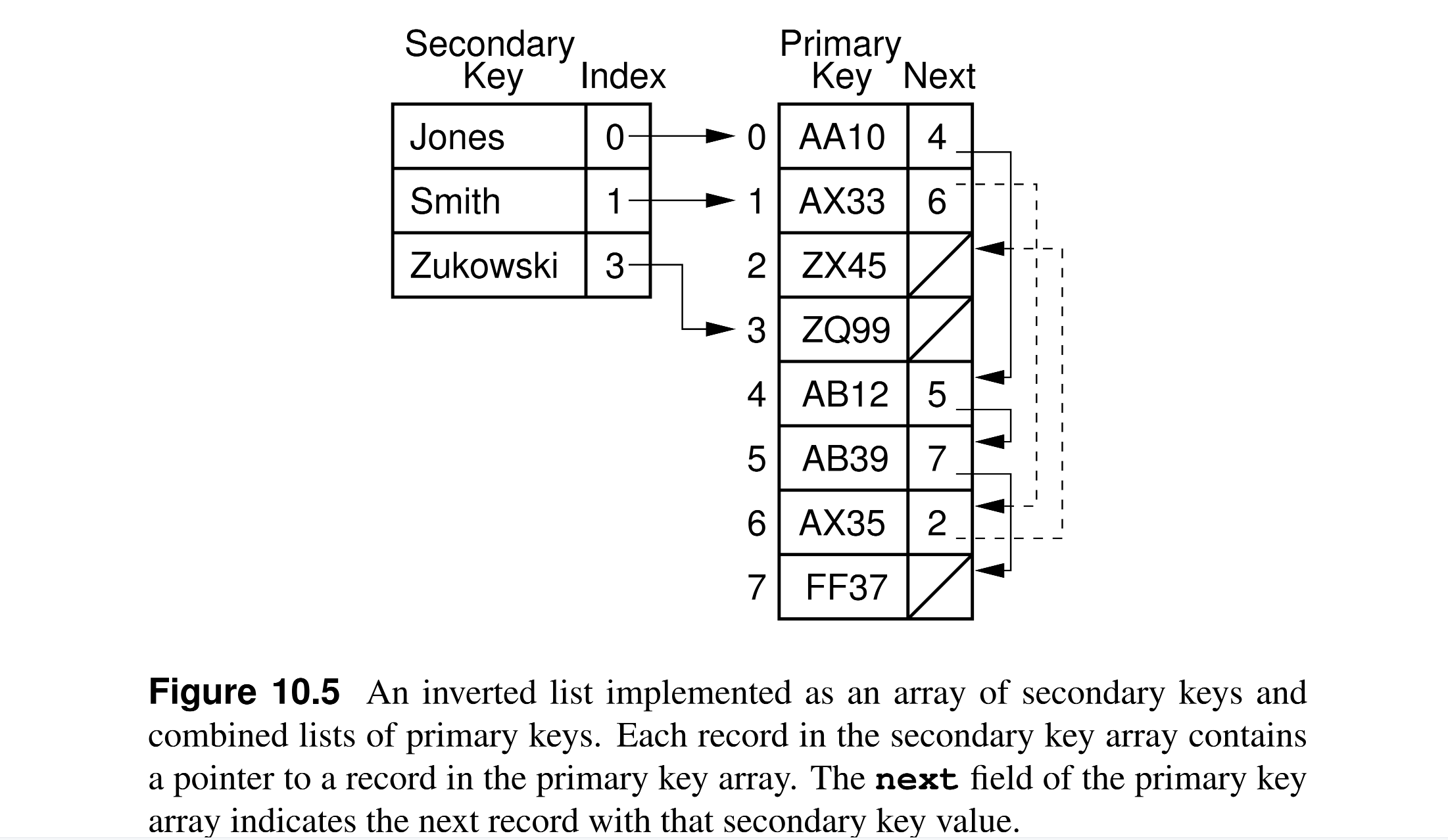
- One solution is to use a two-dimensional array where the first dimension is the secondary key value and the second dimension is a list of primary keys that have this secondary key.
- With no duplications, adding or removing a record to an existing secondary key is cheap, as we only need to update one entry in the index; however, inserting a new secondary key is still expensive as we need to shift all the entries in the index but it is rare compared to the frequency of other operations.
- This approach suffers the array limitations like fixed size, and wasted space for empty slots; thus, each secondary key can point to a linked list of primary keys instead, however, linked lists are not suitable if the index may be stored on disk.

Inverted List
- Secondary indexes also known as inverted lists or inverted files:
- Inverted: because the search works backwards from the secondary key to the primary key to the location of the record to the record itself.
- List: conceptually, every secondary key points to a list of primary keys.
10.2 ISAM
- Linear indexing is not suitable for large databases that require frequent updates as it is a single array that must be sorted after every update; although inverted list reduces this problem, inverted lists are only suitable for secondary indexes with low cardinality (few distinct values, like enums).
- ISAM:
- Is an index was adopted by IBM before the invention of B-trees.
- The problem is that the efficiency of the index is degraded as updates are performed.
- It is a modified version of the linear index that uses a two-level index to reduce the number of disk accesses.
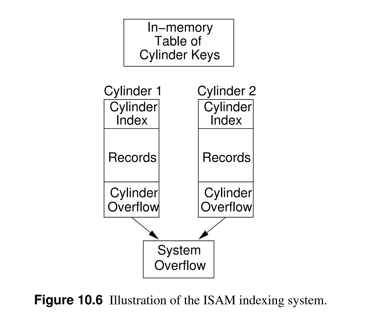
- ISAM uses disk cylinders to efficiently organize data; a disk cylinder is a set of tracks that are at the same distance from the center of the disk but on different platters, thus they can all be read at the same time by setting the disk head at the same position on each platter.
- ISAM structure:
- On disk:
- data is stored on cylinders, where each one holds a section of the list in sorted order (by primary key);
- Each cylinder has an extra space for cylinder overflow.
- Each cylinder has its own index that maps the first/last primary key for each block in the cylinder to the block location within the cylinder.
- In memory:
- a cylinder index is used to map the first/last primary key in a block of the cylinder index to the location of this block on disk.
- On disk:
- When searching:
- The in-memory cylinder index is used to retrieve the block of the internal cylinder index that contains the primary key.
- The internal cylinder index is used to retrieve the exact block that contains the primary key.
- When inserting:
- The record is placed on the correct cylinder’s overflow space.
- Once this space is full, the entire system (all cylinders) is rearranged (sorted).
- Other implementations require periodic sorting of the entire system.
- ISAM was typical of database systems during the 1960s and would normally be done each night or weekly
10.3 Tree-based Indexing
- Linear indexing is efficient when the database is static, that is, when records are inserted and deleted rarely or never.
- ISAM is adequate for a limited number of updates, but not for frequent changes. Because it has essentially two levels of indexing, ISAM will also break down for a truly large database where the number of cylinders is too great for the top-level index to fit in main memory.
- Binary Search Tree is good for implementing primary or secondary indexes, but it may get unbalanced and it is not suitable for on-disk storage (the number of disk accesses will be equal to the height of the tree); even with using buffer pools, BST is not suitable for large on-disk indexes.
- When using trees for indexing, two main issues:
- How to keep the tree balanced?
- How to arrange nodes on blocks to minimize the number of blocks retrieved (disk accesses) on the path from the root to leaves?
- We need a tree that is:
- Automatically remains balanced after updates (inserts and deletes).
- Easy to be stored and retrieved from disk.
- Trees that may satisfy these requirements are:
- AVL trees.
- Splay trees.
- 2-3 trees: its leaves are at the same level always.
- B-trees: the most common tree-based index.
10.4 2-3 Trees
- The structure of a 2-3 tree:
- Each node has either one or two keys.
- Every internal node has either two (if it has one key) or three children.
- All leaves are at the same level.
- If a node has two children (one key):
- Each node in the left subtree has a key less than the key of the node.
- Each node in the center subtree has a key greater than the key of the node.
- If a node has three children (two keys):
- Each node in the left subtree has a key less than the first key of the node.
- Each node in the center subtree has a key greater than the key of the node but less than the second key of the node.
- Each node in the right subtree has a key greater than the second key of the node.

- B-tree features:
- Has at least 2^(h-1) nodes, where h is the height of the tree.
- Has at most 3^(h-1) nodes, where h is the height of the tree.
10.5 B-Trees
- B-trees are usually attributed to R. Bayer and E. McCreight who described the B-tree in a 1972 paper.
- By 1979, B-trees had replaced virtually all large-file access methods other than hashing.
- B-trees Advantages:
- B-trees are always height-balanced, with all leaves at the same level.
- Updates and searches only affects few disk blocks, so the number of disk accesses is minimized.
- B-trees keep related records on the same disk block, so the number of disk accesses is minimized.
- B-trees guarantees that all nodes are nearly full, which makes it space efficient.
- B-tree Structure (of order m):
- Each node is either a leaf or has at least two children.
- Each internal node has between m/2 and m children.
- All leaves are at the same level, so it is always height-balanced.
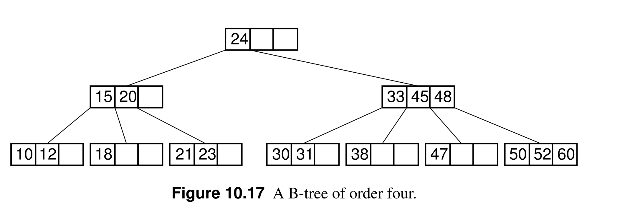
- B-tree is a generalization of 2-3 trees, where each node has m >= 3 children; thus the 2-3 tree is a B-tree of order m=3.
- The B-tree implementations usually have order of 100s which can be contained withing one block, and these blocks usually buffered in memory.
10.5.1 B+-Trees
- The B+-tree is essentially a mechanism for managing a sorted array-based list, where the list is broken into chunks.
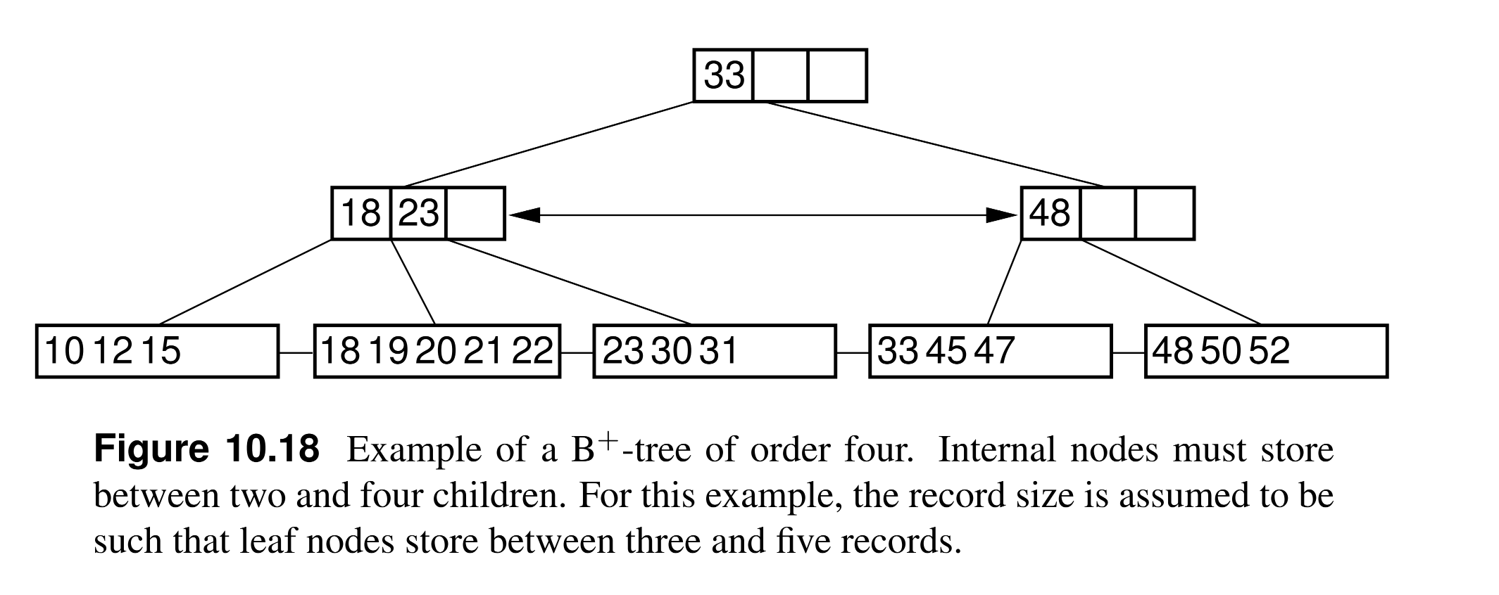
- The most significant difference between the B+-tree and the BST or the standard B-tree is that the B+-tree stores records only at the leaf nodes. Internal nodes store key values, but these are used solely as placeholders to guide the search.
- Leaf nodes store actual records, or else keys and pointers to actual records in a separate disk file if the B+-tree is being used purely as an index.
- The requirement is simply that the leaf nodes store enough records to remain at least half full.
- The leaf nodes of a B+-tree are normally linked together to form a doubly linked list. Thus, the entire collection of records can be traversed in sorted order by visiting all the leaf nodes on the linked list.
- B+-trees are exceptionally good for range queries.
10.5.2 B-Tree Analysis
- The asymptotic cost of search, insertion, and deletion of records from B-trees, B+-trees, and B∗-trees is Θ(log n).
References
-
Shaffer, C. (2011). A Practical Introduction to Data Structures and Algorithm Analysis. Blacksburg: Virginia. Tech. https://people.cs.vt.edu/shaffer/Book/JAVA3e20130328.pdf. Chapter 9: Searching ↩
-
Shaffer, C. (2011). A Practical Introduction to Data Structures and Algorithm Analysis. Blacksburg: Virginia. Tech. https://people.cs.vt.edu/shaffer/Book/JAVA3e20130328.pdf. Chapter 10: Indexing ↩