JA3. Linear Regression Exercises
Exercise 1: Multiple Linear Regression Exercises
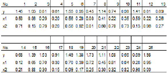
The following measurements have been obtained in a study:

It is expected that the response variable y can be described by the independent variables x1 and x2. This imply that the parameters of the following model should be estimated and tested.
You can copy the following lines to R to load the data:
data1 <- data.frame(
    x1=c(0.58, 0.86, 0.29, 0.20, 0.56, 0.28, 0.08, 0.41, 0.22, 0.35,
             0.59, 0.22, 0.26, 0.12, 0.65, 0.70, 0.30, 0.70, 0.39, 0.72,
             0.45, 0.81, 0.04, 0.20, 0.95),
    x2=c(0.71, 0.13, 0.79, 0.20, 0.56, 0.92, 0.01, 0.60, 0.70, 0.73,
             0.13, 0.96, 0.27, 0.21, 0.88, 0.30, 0.15, 0.09, 0.17, 0.25,
             0.30, 0.32, 0.82, 0.98, 0.00),
      y=c(1.45, 1.93, 0.81, 0.61, 1.55, 0.95, 0.45, 1.14, 0.74, 0.98,
             1.41, 0.81, 0.89, 0.68, 1.39, 1.53, 0.91, 1.49, 1.38, 1.73,
             1.11, 1.68, 0.66, 0.69, 1.98)
)
a. Calculate the parameter estimates \((β_0, β_1, β_2, σ^2)\), in addition find the usual 95% confidence intervals for \(β_0, β_1, β_2\).
we prepare the data and then the model:
model1 <- lm(y ~ x1 + x2, data=data1)
Then we run the summary:
summary(model1)
The output is:
Call:
lm(formula = y ~ x1 + x2, data = data1)

Residuals:
     Min       1Q   Median       3Q      Max
-0.15493 -0.07801 -0.02004  0.04999  0.30112

Coefficients:
            Estimate Std. Error t value Pr(>|t|)
(Intercept) 0.433547   0.065983   6.571 1.31e-06 ***
x1          1.652993   0.095245  17.355 2.53e-14 ***
x2          0.003945   0.074854   0.053    0.958
---
Signif. codes:  0 ‘***’ 0.001 ‘**’ 0.01 ‘*’ 0.05 ‘.’ 0.1 ‘ ’ 1

Residual standard error: 0.1127 on 22 degrees of freedom
Multiple R-squared:  0.9399,    Adjusted R-squared:  0.9344
F-statistic:   172 on 2 and 22 DF,  p-value: 3.699e-14
And according to the summary, the estimates are:
And to find the 95% confidence intervals, we can use the confint function (we can pass the level=0.95 patameter, but it is the default value so we can omit it):
confint(model1)
And the output is:
                 2.5 %    97.5 %
(Intercept)  0.2967067 0.5703875
x1           1.4554666 1.8505203
x2          -0.1512924 0.1591822
So the 95% confidence intervals are:
b. Still using confidence level α = 0.05 reduce the model if appropriate.
We can use the step function to reduce the model:
reduced_model1 <- step(model1, direction="backward", alpha=0.05)
summary(reduced_model1)
And the output is:
Call:
lm(formula = y ~ x1, data = data1)

Residuals:
     Min       1Q   Median       3Q      Max
-0.15633 -0.07633 -0.02145  0.05157  0.29994

Coefficients:
            Estimate Std. Error t value Pr(>|t|)
(Intercept)  0.43609    0.04399   9.913 9.02e-10 ***
x1           1.65121    0.08707  18.963 1.54e-15 ***
---
Signif. codes:  0 ‘***’ 0.001 ‘**’ 0.01 ‘*’ 0.05 ‘.’ 0.1 ‘ ’ 1

Residual standard error: 0.1102 on 23 degrees of freedom
Multiple R-squared:  0.9399,    Adjusted R-squared:  0.9373
F-statistic: 359.6 on 1 and 23 DF,  p-value: 1.538e-15
So the reduced model is:
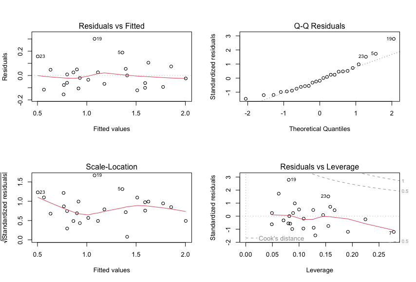
c. Carry out a residual analysis to check that the model assumptions are fulfilled.
We can use the plot function to plot the residuals:
plot(model1)
And the output is:

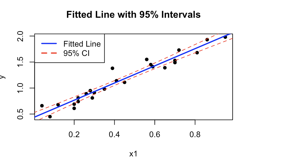
d. Make a plot of the fitted line and 95% confidence and prediction intervals of the line for x1 ϵ [0, 1] (it is assumed that the model was reduced above).
We can use the predict function to predict the values:
x1 <- seq(0, 1, 0.01)
mean_x2 <- mean(data1$x2)
x2 <- rep(mean_x2, length(x1))
newdata <- data.frame(x1=x1, x2=x2)
predictions <- predict(reduced_model1, newdata=newdata, interval="confidence")
And then we can plot the values:
plot(data1$x1, data1$y, pch=16, xlab="x1", ylab="y", main="Fitted Line with 95% Intervals")
lines(newdata$x1, predictions[, "fit"], col="blue", lwd=2)
lines(newdata$x1, predictions[, "lwr"], col="red", lty=2)
lines(newdata$x1, predictions[, "upr"], col="red", lty=2)
legend("topleft", legend=c("Fitted Line", "95% CI"), col=c("blue", "red"), lty=c(1, 2), lwd=2)
And the output is:

Exercise 2: MLR simulation exercise
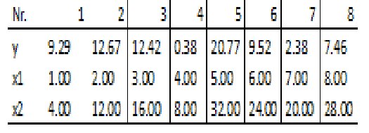
The following measurements have been obtained in a study:

You may copy the following lines into R to load the data
data2 <- data.frame(
     y=c(9.29,12.67,12.42,0.38,20.77,9.52,2.38,7.46),
     x1=c(1.00,2.00,3.00,4.00,5.00,6.00,7.00,8.00),
     x2=c(4.00,12.00,16.00,8.00,32.00,24.00,20.00,28.00)
)
a. Plot the observed values of y as a function of x1 and x2. Does it seem reasonable that either x1 or x2 can describe the variation in y?
# Load data
data2 <- data.frame(
  y=c(9.29,12.67,12.42,0.38,20.77,9.52,2.38,7.46),
  x1=c(1.00,2.00,3.00,4.00,5.00,6.00,7.00,8.00),
  x2=c(4.00,12.00,16.00,8.00,32.00,24.00,20.00,28.00)
)

# Create scatter plots
par(mfrow=c(1,2))  # Arrange plots in a 1x2 grid

# Scatter plot for y vs x1
plot(data2$x1, data2$y, main="y vs x1", xlab="x1", ylab="y", pch=16)

# Scatter plot for y vs x2
plot(data2$x2, data2$y, main="y vs x2", xlab="x2", ylab="y", pch=16)
b. Estimate the parameters for the two models \(Yi = β0 + β1x1,i + єi, єi~N(0,σ2)\) And \(Yi = β0 + β1x2,i + єi, єi~N(0,σ2)\) and report the 95% confidence intervals for the parameters. Are any of the parameters significantly different from zero on a 95% confidence level?
# Fit the model for y ~ x1
fit_x1 <- lm(y ~ x1, data=data2)
conf_intervals_x1 <- confint(fit_x1, level=0.95)

# Fit the model for y ~ x2
fit_x2 <- lm(y ~ x2, data=data2)
conf_intervals_x2 <- confint(fit_x2, level=0.95)

# Display the results
list(conf_intervals_x1=conf_intervals_x1, conf_intervals_x2=conf_intervals_x2)
And the output is:
$conf_intervals_x1
                 2.5 %    97.5 %
(Intercept) -0.5426374 24.897637
x1          -3.1447959  1.893129

$conf_intervals_x2
                 2.5 %     97.5 %
(Intercept) -7.5580921 15.9659492
x2          -0.2957889  0.8688246
So the 95% confidence intervals are:
We notice that \(B_0\) at 95% is significantly different from zero, while the other three numbers are relatively close to zero.