JA7- Absenteeism in School (Multiple Regression Example)
Statement
A study was conducted on absenteeism in school and the data was procured. Use the collected data to answer the following questions (Data: absenteeism.csv).
- a. Import the dataset in JASP and run the regression where days is the dependent variable and the explanatory variables (factors) are:- eth (0- aboriginal, 1- not aboriginal), sex (0- female, 1- male) and lnr (0 – average learner, 1- slow learner). Show the full output from JASP.
- b. Write the equation of the regression model
- c. Interpret each one of the slopes in this context. Determine if each of the slopes are statistically significant based on the p-value for an alpha significance of 5%.
- d. Calculate the residual for the second observation in the data set.
- e. What is the model adjusted R-squared value? Interpret it.
Answer
Regression Analysis Process Using JASP
Here is a step by step guide to the analysis performed in JASP, following the guide by Research By Design (2020):
- Convert the data to a CSV file:
- The data is provided as a
xlsxfile, which is not directly compatible with JASP. We need to convert it to acsvfile. - I opened the file in Excel and saved it as a
csvfile namedabsenteeism.csv.
- The data is provided as a
- Load the data into JASP:
- Use
File > Openfrom the top menu. - Select
Computerand thenBrowse. - Select the dataset file.
- Use
- Configure the fields:
- The dataset has the following fields
days,eth,sex,age, andlnr. - The
eth,lnr, andsexvariables are categorical, and not numerical; we need to associate a number to each category. - Fix the
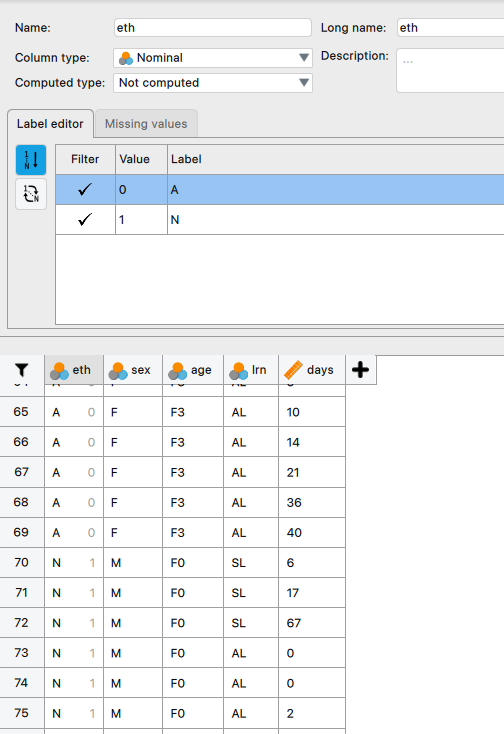
eth(ethnicity) variable:- The
ethvariable has two categories:aboriginal(A) andnot aboriginal(N). - Aboriginal = A = 0.
- Not Aboriginal = N = 1.
- Double click on the
ethcolumn name to open theVariable Properties. - Select
NominalunderVariable Role. - Update the
Valuesto0 = A, 1 = N, according to Image 1 below.
- The
- Fix the
sexvariable:- The
sexvariable has two categories:female(F) andmale(M). - Female = F = 0.
- Male = M = 1.
- We update the
sexvariable as we did with theethvariable above.
- The
- Fix the
lnrvariable:- The
lnrvariable has two categories:average learner(A) andslow learner(S). - Average learner = A = 0.
- Slow learner = S = 1.
- The
- Fix the
agevariable:- The
agevariable has 4 categories:F0,F1,F2, andF3. - F0 = 0, F1 = 1, F2 = 2, F3 = 3.
- The
- The dataset has the following fields
- Do the Regression analysis:
- Use
Regression > Classical > Linear Regressionfrom the top menu. - Dependent variable is the
yvariable which isdays. - Covariate is the
xvariable, which areeth,sex, andlnr(added in order). - Set the
MethodtoEnter. - Under
Statistics:- Select
Regression Coefficient > Confidence intervals. - Select
Regression Coefficient > Descriptives. - Select
Residuals > Statisticsto check for outliers and influential points (Std. Residuals should be between -3 and 3). - Select
Residuals > Durbin-Watsonto check for independence of observations (Durbin-Watson statistic should be between 1 - 3).
- Select
- Under
Plots:- Select
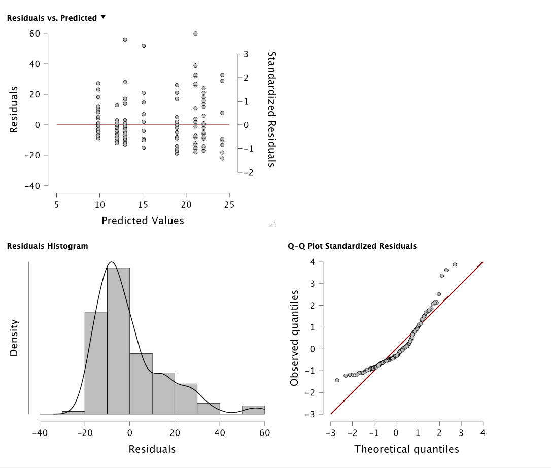
Residuals plots > Residuals vs Histogramto check for normality. - Select
Q-Q plot standardized residualsto check for normality. - Select
Residuals vs predictedto check for homoscedasticity.
- Select
- Use
Image 1: Variable Properties for eth |
|---|
 |
Results of the Analysis
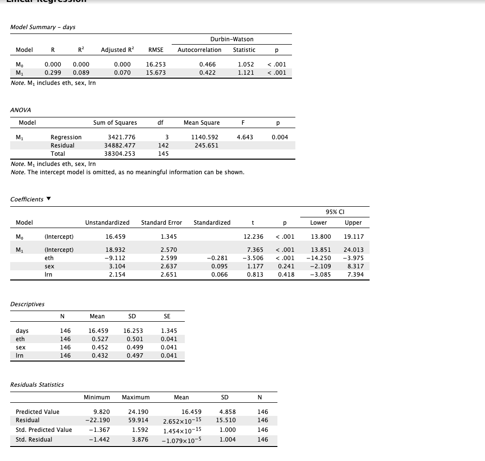
We have loaded the data into JASP and performed the linear regression analysis. The results are as follows:
| Image 2: Linear Regression Output |
|---|
 |
| Image 3: Linear Regression Output (2) |
|---|
 |
A. Import the dataset in JASP and run the regression where days is the dependent variable and the explanatory variables (factors) are:- eth (0- aboriginal, 1- not aboriginal)
The regression analysis was performed in JASP with the dependent variable days and the explanatory variables eth, sex, and lnr. The output is shown in the images (2 and 3) above.
B. Write the equation of the regression model
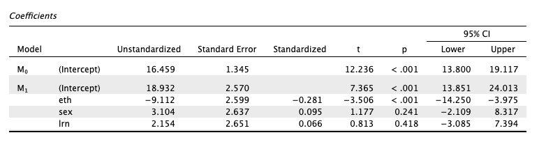
Looking at the coefficients table in the output, shown in the Image 4 below:
| Image 4: Coefficients Table |
|---|
 |
The general form of the regression equation is:
From the table, the coefficients are:
| Coefficient | Name | Value |
|---|---|---|
| \(\beta_0\) | Intercept | 18.932 |
| \(\beta_1\) | eth | -9.112 |
| \(\beta_2\) | sex | 3.104 |
| \(\beta_3\) | lnr | 2.154 |
Therefore, the regression equation is:
C. Interpret each one of the slopes in this context. Determine if each of the slopes are statistically significant based on the p-value for an alpha significance of 5%
Looking at the coefficients table in the output, shown in the Image 4 below:
| Image 4: Coefficients Table |
|---|
|
From the table, the coefficients are:
| Coefficient | Name | Value | P-value | Significant | Correlation |
|---|---|---|---|---|---|
| \(\beta_0\) | Intercept | 18.932 | 0.001 | Yes | - |
| \(\beta_1\) | eth | -9.112 | 0.001 | Yes | Negative |
| \(\beta_2\) | sex | 3.104 | 0.241 | No | Positive |
| \(\beta_3\) | lnr | 2.154 | 0.418 | No | Positive |
Here is the interpretation of the slopes:
- Ethnicity: (1 for not aboriginal, 0 for aboriginal):
- For every unit increase in the
ethvariable (from aboriginal to not aboriginal), the number of days absent decreases by 9.112 days due to the negative sign. - The slope is statistically significant (p-value = 0.001).
- Thus, not aboriginal students (higher
ethvalue) tend to have fewer days absent compared to aboriginal students. - Specifically, Not Aboriginal students are expected to be absent for 9.112 days less (on average) than Aboriginal.
- For every unit increase in the
- Sex: (1 for male, 0 for females):
- For every unit increase in the
sex(from females to males), the number of days absent increases by 3.104 days due to the positive sign. - The slope is not statistically significant (p-value = 0.241).
- Thus, there is no significant difference in the number of days because we cannot reject the null hypothesis (p-value > 0.05).
- However, if we would tolerate a higher Type I error rate, the data shows that males tend to be absent for more days (3.104 days on average) than females.
- For every unit increase in the
- Learner Type: (1 for slow learner, 0 for average learner):
- For every unit increase in the
lnrvariable (from average to slow learner), the number of days absent increases by 2.154 days due to the positive sign. - The slope is not statistically significant (p-value = 0.418).
- Thus, there is no significant difference in the number of days because we cannot reject the null hypothesis (p-value > 0.05).
- However, if we would tolerate a higher Type I error rate (very unlikely), the data shows that slow learners tend to be absent for more days (2.154 days on average) than average learners.
- For every unit increase in the
D. Calculate the residual for the second observation in the data set
The residuals are the differences between the observed values and the predicted values. The second observation in the dataset is (O2)
| Ethnicity | Sex | Age | Learner Type | Days |
|---|---|---|---|---|
| A=0 | M=1 | F0=0 | SL=1 | 11 |
Let’s compute the days for the scend observation (O2) using the regression equation:
The residual for the second observation is:
Thus, the residual for the second observation is -13.19.
E. What is the model adjusted R-squared value? Interpret it
| Image 6: Model Summary |
|---|
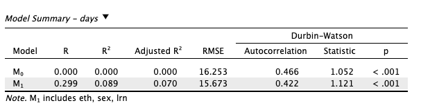 |
The adjusted R-squared value is a measure of how well the independent variables explain the variance in the dependent variable. It adjusts the R-squared value for the number of predictors in the model and the degrees of freedom.
The R^2=0.089 and the Adjusted R^2=0.070 in the according to the image above. We will interpret the adjusted R-squared value as is more reliable when there are multiple predictors in the model.
Here are some notes about the interpretation:
- Only 8% of the variance in the dependent variable
daysis explained by the independent variableseth,sex, andlnr. - There is a
1%difference between the R-squared and the adjusted R-squared values, which indicates that adding the predictors did not significantly improve the model. - The low adjusted R-squared value suggests that the entire model is questionable as it does not explain much of the variance in the dependent variable.
- Maybe trying to add/remove one or more predictors will yield a better Adjusted R-squared value, hence, a better model.
References
- Research By Design. (2020, June 5). How to do simple linear regression in JASP (14-7) [Video]. YouTube. https://youtu.be/vKGphOrzze8