2. Algorithm Analysis
3. Algorithm Analysis 1
- Asymptototic algorithm analysis:
- Is a method to compare the resource consumption of two algorithms.
- It does not show slight differences in resource consumption, but it flags the significant differences.
- It is an estimation of the cost of an algorithm.
- It measures the efficiency of an algorithm or its implementation (program) as the input size grows.
- It analyzes:
- The time required for an algorithm to run (or an instantiation of an algorithm into a program to execute).
- The space required for a data structure.
-
Largest-value sequential search:
/** @return Position of largest value in array A */ static int largest(int[] A) { int currlarge = 0; // Holds largest element position for (int i=1; i<A.length; i++) // For each element if (A[currlarge] < A[i]) // if A[i] is larger currlarge = i; // remember its position return currlarge; // Return largest position } -
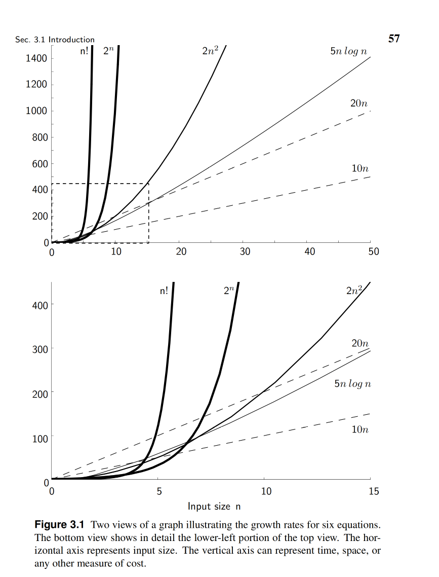
The growth rate for an algorithm is the rate at which the cost of the algorithm grows as the size of its input grows.
- Growth rates (sorted from fastest to slowest):
- Linear: \(O(n)\) or \(c \cdot n\) where \(c\) is a constant. Practically, the value of \(c\) is not important.
- Logarithmic: \(O(n \space log n)\) or \(n \space log n\).
- Quadratic: \(O(n^2)\) or \(n^2\).
- Exponential: \(O(2^n)\) or \(2^n\).
- Factorial: \(O(n!)\) or \(n!\).

- Notes:
- comparing \(c1 ⋅ n\) and \(c2 ⋅ n\) gives the same comparison as comparing \(n\) and \(n\). So, we can ignore the constant \(c1\) and \(c2\).
- \(n^a\) grows faster than \(log^a(n)\) or \(log (a^n)\) => Quadratic grows faster than logarithmic.
- \(a^n\) grows faster than \(n^a\) where \(n\) is the input size and \(a\) is a constant => Exponential grows faster than quadratic.
- When running an algorithm, there are three cases:
- Best case. The input is the smallest possible input. Ignored in practice, but there are rare cases where analyzing the best case is important.
- Average case. When running the algorithm a large number of times on a randomized input. If the program is expected to run a huge number of times on different inputs, then the average is the most representative of the algorithm’s performance, and analyzing it is important.
- Worst case. The input is the largest possible input.
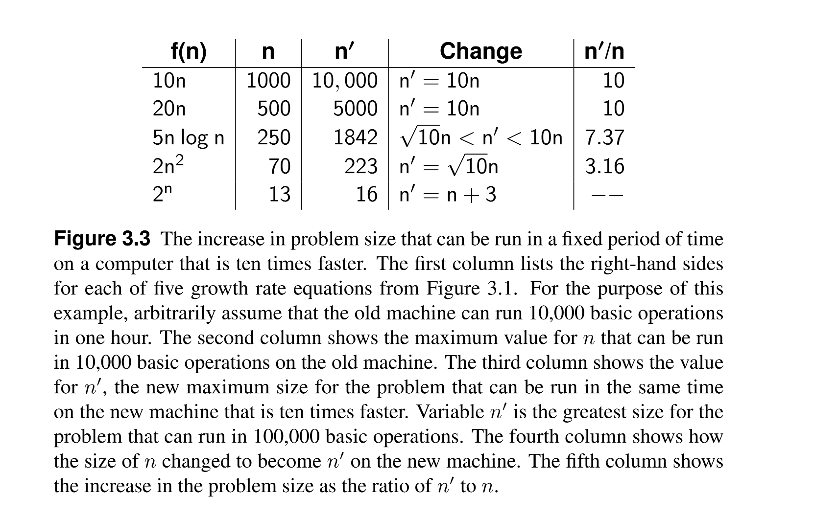
- How using a 10X computer affects the running time of an algorithm:
- Linear: 10X computer => 10 times faster.
- Logarithmic: 10X computer => between \(\sqrt{10}\) and \(10\) times faster.
- Quadratic: 10X computer => \(\sqrt{10}\) times faster.
- Exponential: 10X computer => no change.
- So using a 10X computer only improves the running time of linear and logarithmic algorithms. For quadratic and exponential algorithms, the running time is not improved.
- The image below compares running times in 1x and 10x computers for different algorithms:

- Do NOT change the computer to improve the running time of an algorithm, change the algorithm instead.
3.4 Asymptotic Analysis
- The Upper bound:
- It indicates the highest growth rate of an algorithm.
- It is the growth rate value for the
highestvalue in the worst-case range. - We say: “This algorithm has an upper bound to its growth rate of \(n^2\) in the average case”.
- Described by the big-O notation or \(O\) notation.
- Big-Oh notation: \(O(f(n))\) describes an upper bound and lower bound to its growth.
- There is no strict equality in the big-Oh notation. We say that growth is in \(O(f(n))\), and not growth is \(O(f(n))\) or growth = \(O(f(n))\).
- The Lower Bound:
- It indicates the least amount of resources required to run an algorithm in its worst case.
- It is the growth rate value for the
lowestvalue in the worst-case range. - Described by the big-omega notation or \(\Omega\) notation which is similar to the big-Oh notation.
- The Theta Notation or \(\Theta\) notation:
- It indicates the exact growth rate of an algorithm (where the upper bound and lower bound are equal).
- It is the intersection of the big-Oh and big-omega notations or the middle of the range of the worst-case growth rate (lower bound and upper bound).
- It indicates no meaningful difference between the upper bound and lower bound growth rates.
- It is better to use the Theta notation than the big-Oh notation because it is more precise.
- The importance of lower and upper bounds becomes more important when we have little knowledge about the algorithm, and less important -in favor of the Theta notation- when we have more knowledge about the algorithm.
- The worst, average, and best cases are not the same as the upper, lower, and theta bounds:
- The worst, average, and best cases describe ranges of values for the input size; and are represented by a set of sets of inputs.
- The upper, lower, and theta bounds describe growth rates for an input range; and are represented by Big-Oh, Big-omega, and Theta notations.
- Rules:
- Transitivity: \(f(n) = O(g(n)), g(n) = O(h(n)) ⇒ f(n) = O(h(n))\).
- Constants are ignored: \(f(n) = O(c \cdot g(n)) ⇒ f(n) = O(g(n))\).
- When adding two functions, the highest growth rate is kept: \(f(n) = O(g(n)) + O(h(n)) ⇒ f(n) = f1 + f2 = O(max(f1, f2))\).
- When multiplying two functions, the growth rate is multiplied: \(f(n) = O(g(n)) \cdot O(h(n)) ⇒ f(n) = f1 \cdot f2 = O(f1 \cdot f2)\).
3.5 Calculating the running time of a program
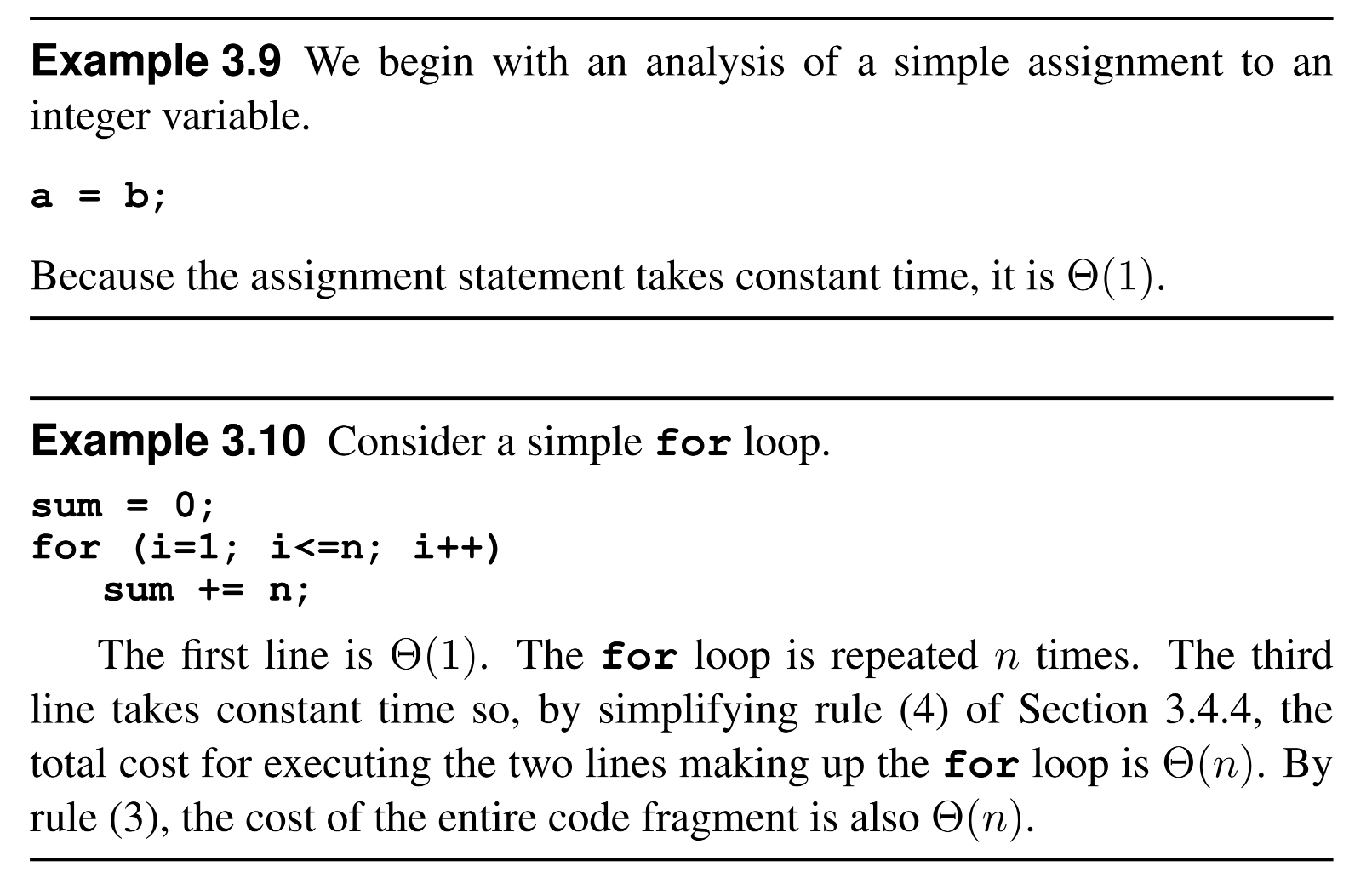
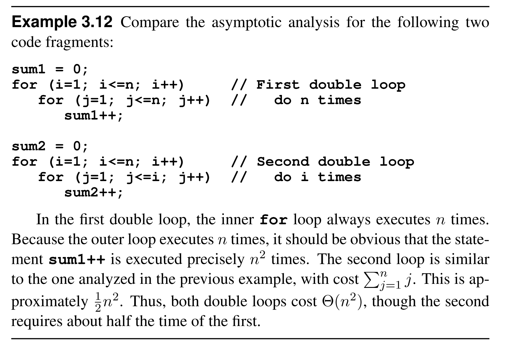
- The Big-Oh values for code that run in sequential order is + (added) while code that is trapped or called within another code (e.g. a loop) is x (multiplied).
- Loops that increment by 1 e.g. ++1 are linear and have a growth rate of \(O(n)\).
- Loops that increment by multiplying by 2 e.g. *= 2 are logarithmic and have a growth rate of \(O(log n)\).
- \(O(n.log(n))\) is always greater than \(O(n)\) which means \(O(n)\) algorithms are always faster than \(O(n.log(n))\) algorithms.
- Examples:


Recurrences 2
- Recursion is breaking down an object into smaller objects of the same type.
- Recurrence equation describes the value of a function in terms of the values of the function at smaller inputs.
- Reoccurrence equation for Tower of Hanoi problem:
T(1) = 1
T(n) = 2T(n-1) + 1  (for n >= 2)
- Guess-and-Verify is method that is used to solve recurrence equations:
- Guess the solution.
- Verify the guess using mathematical induction.
- Looking at the recurrence equation for Tower of Hanoi problem, we can guess that the solution is \(T(n) = 2^n - 1\) and then verify it using mathematical induction.
Claim:
    if:
        T(1) = 1
        T(n) = 2T(n-1) + 1 (for n >= 2)
    then:
        T(n) = 2^n - 1

Proof:
    Let P(n) be the statement that T(n) = 2^n - 1
    Base Case:
        P(1) = T(1) = 2^1 - 1 = 1
        P(1) is true
    Inductive Step:
        Assume P(n) is true for some n >= 1 and prove P(n+1)  for n >= 1
        T(n+1) = 2T(n) + 1  // replace T(n) with 2^n - 1 as it is assumed true
               = 2(2^n - 1) + 1
               = 2*2^n - 2 + 1
               = 2^(n+1) - 1
        P(n+1) is true

Conclusion:
    By the principle of mathematical induction, P(n) is true for all n >= 1
Extra resources
References
-
Shaffer, C. (2011). A Practical Introduction to Data Structures and Algorithm Analysis. Blacksburg: Virginia. Tech. https://people.cs.vt.edu/shaffer/Book/JAVA3e20130328.pdf. Chapter 3. ↩
-
Srini Devadas & Eric Lehman (2005). Mathematics for Computer Science. 6.042/18.062J. Lecture Notes March 17, 2005. https://dspace.mit.edu/bitstream/handle/1721.1/104427/6-042j-spring-2005/contents/lecture-notes/l12_recur2.pdf ↩